Concepts
ISO 13943:2023 defines human behaviour in fire as “actions performed in the event of a fire as a result of a behavioural or decision-making process”. The talk A Modular Workflow for Visibility-Aware Evacuation Modelling (Visibility Seminar 2026) splits the behaviour that smoke disturbs into three questions. Speed asks how fast an occupant can walk. Route choice asks which exit the occupant heads for. Wayfinding asks which exits the occupant knows about at all. pyFDS-Evac answers each question from the output of a finished Fire Dynamics Simulator (FDS) run and hands the answers to JuPedSim, which moves the agents.
This page gives the intuition behind each answer and the rules you need to read a result. The published laws the answers rest on, in their authors' notation, are on the Fundamentals pages. How the code implements them, with its defaults and its departures from the literature, is on the Models pages.
pyFDS-Evac is research software, provided without warranty. It is not intended for regulatory or design use. See Limitations.
One-way coupling and the data flow
FDS runs once, before any agent moves, and pyFDS-Evac only reads the slice files it stored. This is one-way coupling: a crowd that blocks a door does not change the smoke that reaches it. In return, one fire can serve any number of egress runs, and a prescribed field can replace FDS entirely, as in the Quickstart.
FDS output (.smv + slice files)
  │
  ├─ fdsreader ─ SliceFieldSampler ─┬─ ExtinctionField   K [1/m]
  │   nearest-neighbour lookup      ├─ FdsFedField       CO, CO₂, O₂, irritants
  │   of (t, x, y) at one height    └─ FdsHeatField      gas temperature [°C]
  │
  └─ fdsvismap ─ VisibilityModel     which cells can read which sign, per time
                                   │
Scenario (load_scenario) ──────────┤
                                   ▼
                             run_scenario()  ── JuPedSim moves the agents
                                   │
                                   ▼
  trajectory (SQLite) + optional per-agent histories (smoke, FED, route,
  route cost, cognitive map) + <trajectory>.manifest.json
The sampler takes the nearest stored value on a slice. Every quantity —
extinction, each gas, temperature, and the extinction slice fdsvismap uses
for sign legibility — is read from the horizontal slice nearest
--smoke-slice-height (1.6 m by default), the same height for every agent
(FDS slice sampling). The manifest records the package versions, the
seed, the scenario and the FDS version, so a result can be traced to the code
and the fire that produced it. The walkthrough runs this
chain on a tracked case, and Your FDS case
lists the slices the deck must write.
Speed
From extinction to walking speed
Smoke enters the speed model through the extinction coefficient K [1/m],
read from the FDS SOOT EXTINCTION COEFFICIENT slice at the agent’s position.
Each agent keeps its own unimpeded speed \(v_0\) and walks at a fraction of it,
where the speed factor \(f\) falls from 1 in clear air towards a floor in
dense smoke. The default is the linear Frantzich–Nilsson law in the fractional
form and with the constants of FDS+Evac, so a difference between the two tools
downstream of speed cannot come from the speed law. The alternative is the
fridolf option, the law of Fridolf et al. (2019, Eq. 7)
in the sighting distance
\(V = C/K\): above 3 m the speed is unchanged, below it drops by 0.34 m/s per
metre, to an absolute floor of 0.2 m/s. Being additive, its factor depends on
each agent’s \(v_0\). It is available only from Python (see the parameter split). The published laws are on
Walking speed in smoke; the coded forms are
on the smoke-speed model page.
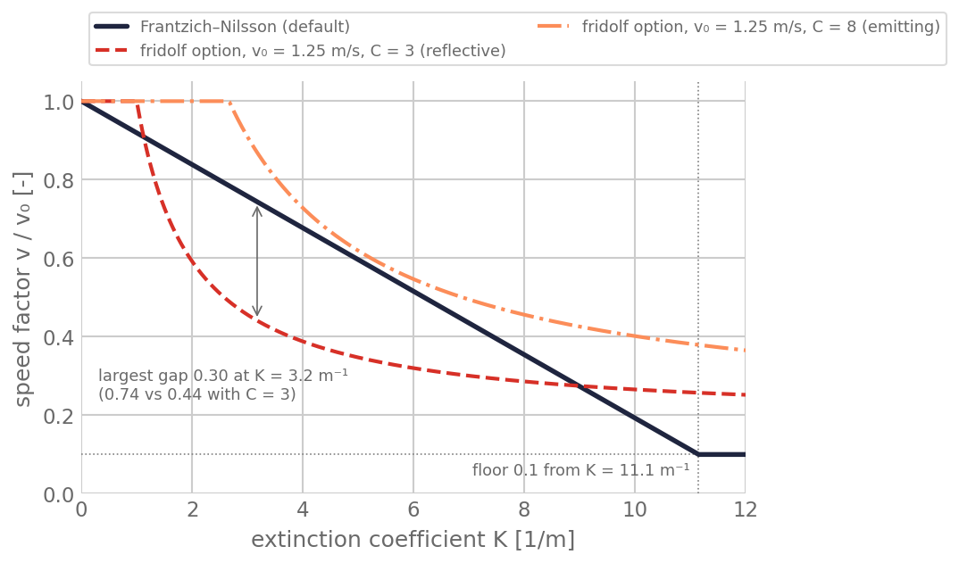
Figure 1. Speed factor \(v/v_0\) [-] against K [1/m]. Solid dark blue:
Frantzich–Nilsson at the defaults, with its floor. The fridolf option at
\(v_0\) = 1.25 m/s with \(V = C/K\): red dashed for C = 3, orange dash-dotted
for C = 8. The arrow marks the largest gap between Frantzich–Nilsson and C = 3. Script: scripts/figures/speed_laws.py.
Tenability: a brake and a stop
Some effects of smoke depend only on what the agent meets now; others accumulate into a dose. pyFDS-Evac keeps them apart: speed follows what the agent meets at the moment, and a dose acts only as a switch:
$$ v_i = v_{0,i}\; f(K)\; g(\mathrm{FIC})\; \mathbb{1}\!\left[\mathrm{FED}_i < D_i\right]\; \mathbb{1}\!\left[\mathrm{FED}_{\mathrm{heat},i} < D_{\mathrm{heat},i}\right]. $$The brake is \(f(K)\,g(\mathrm{FIC})\). The fractional irritant concentration
(FIC) sums the irritant gases, each over a reference concentration, and \(g\)
lowers the speed further as it rises, down to a floor. \(g = 1\) unless
--enable-fic-speed is given: FDS+Evac has no irritant slowdown, so it is
off by default. FIC is a concentration,
not a dose, so \(g\) follows the gas where the agent stands. One quirk: when
FIC drops to exactly zero the factor is not recomputed, so an agent that walks
out of a plume into clean air keeps its last slowdown
(#142).
The stop is the fractional effective dose (FED). The toxic-gas dose follows
the Purser sum as FDS+Evac computes it, which adds irritants into the dose,
unlike ISO 13571. With --enable-heat-fed, convective heat from an FDS
TEMPERATURE slice accumulates in a second dose (ISO 13571:2012 Eq. (9),
fully clothed, by default). The heat dose is off by default, as FDS+Evac has
none. The two doses are never added. By default every agent stops at FED = 1,
as FDS+Evac does; with --incapacitation-mode probabilistic each agent draws
its own threshold, so a population does not stop all at once. When either dose
crosses its threshold, the agent’s speed is set to zero and it stays in place
as an obstacle for the rest of the run. It is never counted as evacuated, and
its dose record stops at the collapse. Dead agents stay because agents that
collapse just short of an exit block it for others; removing them would be
wrong. When no mobile agent is left and no flow window is open, the run ends
(Reading the results).
--disable-tenability turns off the slowdown and both stops,
while the doses are still logged.
Two consequences matter when you read a result. An FED below the threshold
leaves the walking speed unchanged, however close it comes. And the heat dose
only incapacitates: it neither slows agents nor affects route choice, and
radiant heat from a hot layer enters only with the opt-in --heat-regime layer or --heat-radiant-source integrated-intensity, and from a flame or
hot surfaces only with the latter, with a user factor. The published dose laws are on
Asphyxiant fractional effective dose,
Irritant gases, Heat
and Incapacitation thresholds.
The coded forms are on the FED model page.
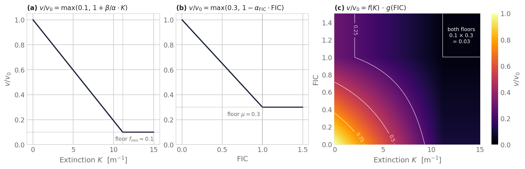
Figure 2. The brake: (a) f(K), (b) g(FIC) and (c) their product, with
contours of equal speed factor. The irritant factor g has no known source
and is off by default; the published relation is Eq. 63.13 on
Irritant gases.
FED does not appear on
these axes; it only sets the speed to zero at the agent’s threshold.
Script: scripts/generate_tenability_curves.py.
Route choice
Routes live on a stage graph
Routes are paths on a directed graph whose nodes are the spawn areas, checkpoints and exits. Each edge carries a polyline that JuPedSim computes along the walkable area, so it follows the corridors, not a straight line through walls. Smoke is read once in every grid cell of the FDS slice that the polyline crosses, and the mean of the samples, \(\bar K_{uv}\), is a discrete Beer–Lambert mean (see Extinction coefficient) taken along a walked path instead of a line of sight.
A route is measured from where the agent stands. Its mean extinction \(\bar K_k\) is the length-weighted mean over its edges, and \(L_k\) is the distance still to walk. Each agent re-decides at a fixed interval, and a decision is not remembered: every re-decision starts again from the current field. pyFDS-Evac sets each agent’s target itself and JuPedSim walks the agent there; see How agents are steered.
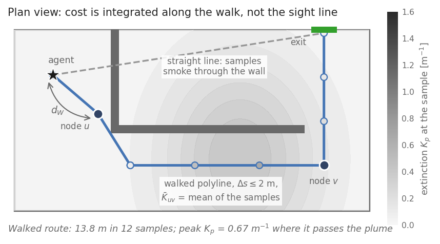
Figure 3. Schematic with a toy extinction field, not a simulation. The
straight line (dashed) passes through a wall; the walked polyline (solid) goes
around it, read once in each cell of a notional 0.5 m FDS grid that it
crosses, its samples coloured by K [1/m] at the time the agent would reach
them. \(d_W\) is the walkable distance to the first node.
Script: scripts/figures/stage_graph.py.
The exposure gate
Under the default "gate" cost model, one quantity carries all of the smoke
reasoning: the optical depth along the walk, \(\tau_k = \bar K_k L_k\), the
column of smoke the agent would pass through.
First, a shortest-path search from the agent’s position finds one path to each exit, with every edge weighted by its own optical depth at decision time: the least-smoky path, which in clear air is the shortest. The first leg is the walk from the agent to the route’s first node, charged for the smoke ahead of the agent. Second, each candidate is re-evaluated with anticipation, each edge sampled at the time the agent would reach it. By default the router sees the whole future of the fire, so the result is an upper bound on how well an occupant could route. Third, the gate refuses a route whose \(\tau\) exceeds a budget \(\tau_{\max}\), or whose projected dose at arrival exceeds a fixed limit. The survivors are ranked by \(\tau\), and travel time breaks ties, so in clear air the model reduces to the nearest exit.
Because \(\tau\) contains the distance, a long clean route can beat a short smoky one, but a slightly cleaner route cannot divert an agent for free. A rival exit is held to a stricter budget than the current one, and the current exit gets a discount in the ranking. If every route is refused, the agent still moves and takes the least smoky one. Irritants and heat do not enter route choice: FIC and the gate respond to the same smoke, so routing on both would count it twice.
The budget is inherited from the door rule of FDS+Evac, which rests on Jin’s
visibility law (see Visibility through smoke).
Here it bounds smoke integrated along a walked path, which measures exposure,
not sight. It is cited, not calibrated, and FDS+Evac ranks on smoke only as a
last resort, so the gate departs from FDS+Evac rather than reproducing it. The
routing page gives the defaults, the derivation of the
budget, the "additive" alternative and a measured case of oscillation.
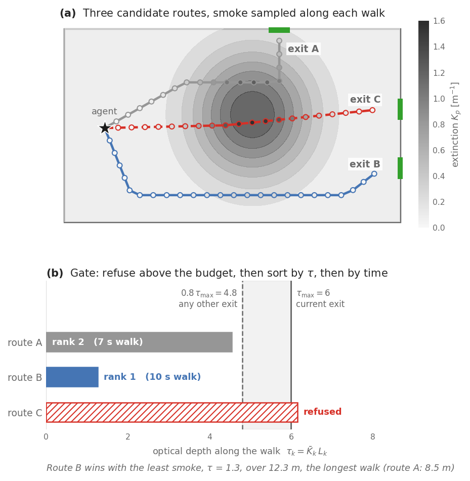
Figure 4. Schematic with a toy plume, not a simulation. Top: three candidate
routes, their samples shaded by K [1/m]. Bottom: their optical depth \(\tau\) against the
budget (the same for every exit). Route C is refused; route B ranks first although it is the longest
walk. Script: scripts/figures/exposure_gate.py.
Wayfinding
Route choice picks among the exits an agent knows. Wayfinding decides which exits those are. The code, its defaults and its limitations are on Models › Wayfinding. A walk-through in the order of the talk, with the examples, is on Wayfinding in practice.
Knowing is not seeing
Each agent carries a cognitive map: the part of the building’s route graph it knows. The map is a data structure, not a psychological construct. It starts with whatever the agent’s familiarity gives it:
- Fully familiar (the default): the whole graph, by assumption.
- Discovery: only its spawn area, plus the neighbouring places whose signs can be read from the spawn area’s routing point (the same point for everyone spawning there).
- A number between 0 and 1: each exit is known from the start with that probability, so a crowd can be a mixture rather than two groups.
entrance: names one exit that is also known from the start, such as the door the agent came in by. It must be an exit reachable from the spawn area; otherwise it is ignored without a warning.
After that, the map grows only when the agent can read a sign (a run with visibility switched off lets it learn by contact instead). A sign is legible from where the agent stands when three conditions hold:
- the agent is on the side the sign faces (a sign without a bearing is readable from every side);
- no wall stands between them;
- the smoke along the line of sight leaves enough visibility, by Jin’s law, to cover the distance.
For a sign with a bearing, the more obliquely it is seen, the more visibility it needs. Legibility is precomputed for the whole floor, from the fire’s smoke or from clear air, and the run only looks it up.
When a neighbouring place’s sign becomes legible, that place is added to the map. Being legible is a state of the moment. Being known lasts.
Routing on what is known
The router ranks only routes over places the agent knows. An exit the agent
has not learned is not a rejected option; for the router, it does not exist.
If no known exit is reachable, the spawn area’s no_known_exit decides. By
default the agent follows a default route, as in FDS+Evac: the journey of its
spawn area, or without one the exit nearest it on foot. That exit need not be
in its map, and the exit history flags it when the agent leaves through it
(#610). With
explore, the agent heads instead for a known place it has not been to yet,
and when none is left, it walks between the places it knows, hoping to see a
new sign on the way; with nowhere known to go it stands.
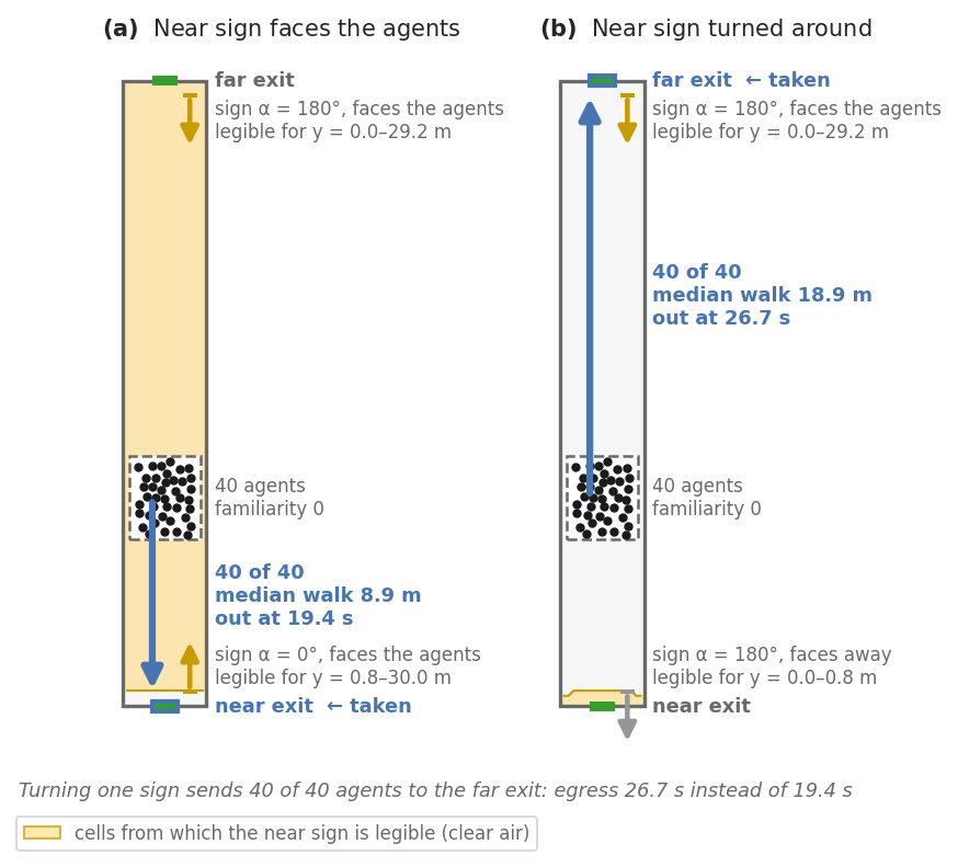
Figure 5. One number flips the exit. A corridor with an exit at
each end and 40 agents at familiarity 0. Only the bearing of the near exit’s
sign differs. Yellow cells are those from which the near sign is legible.
Facing the agents, the near exit is learned and taken; facing away, it is
never learned and the agents walk to the far one. Script:
scripts/figures/sign_bearing.py.
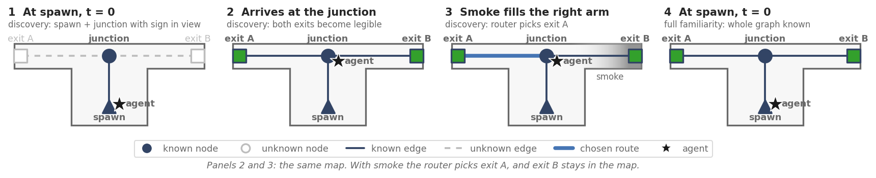
Figure 6. Schematic, drawn by hand, not a simulation. Filled nodes and solid
edges are known. (1) At spawn, a discovery agent knows the junction, whose sign
is legible. (2) At the junction, both exits are learned. (3) Smoke fills the
right arm. Exit B stays known; the router judges its route by the smoke on it,
not by its sign. (4) A fully familiar agent knows everything at t = 0. Script:
scripts/figures/cognitive_map.py.
The map remembers
A place stays known after its sign is hidden again by distance, angle, a wall or smoke. Knowing an exit does not mean choosing it: the router still compares it with the other known exits from where the agent stands. Memory shows when the agent is somewhere it cannot read the sign. There it can still choose the exit it learned earlier. Without the memory, the same place would give a different choice.
The map limits what an agent knows of the building, not what it knows of the smoke. Once it knows an exit, the router prices the whole route to it with the smoke field of the fire, including stretches the agent has never seen (#125).
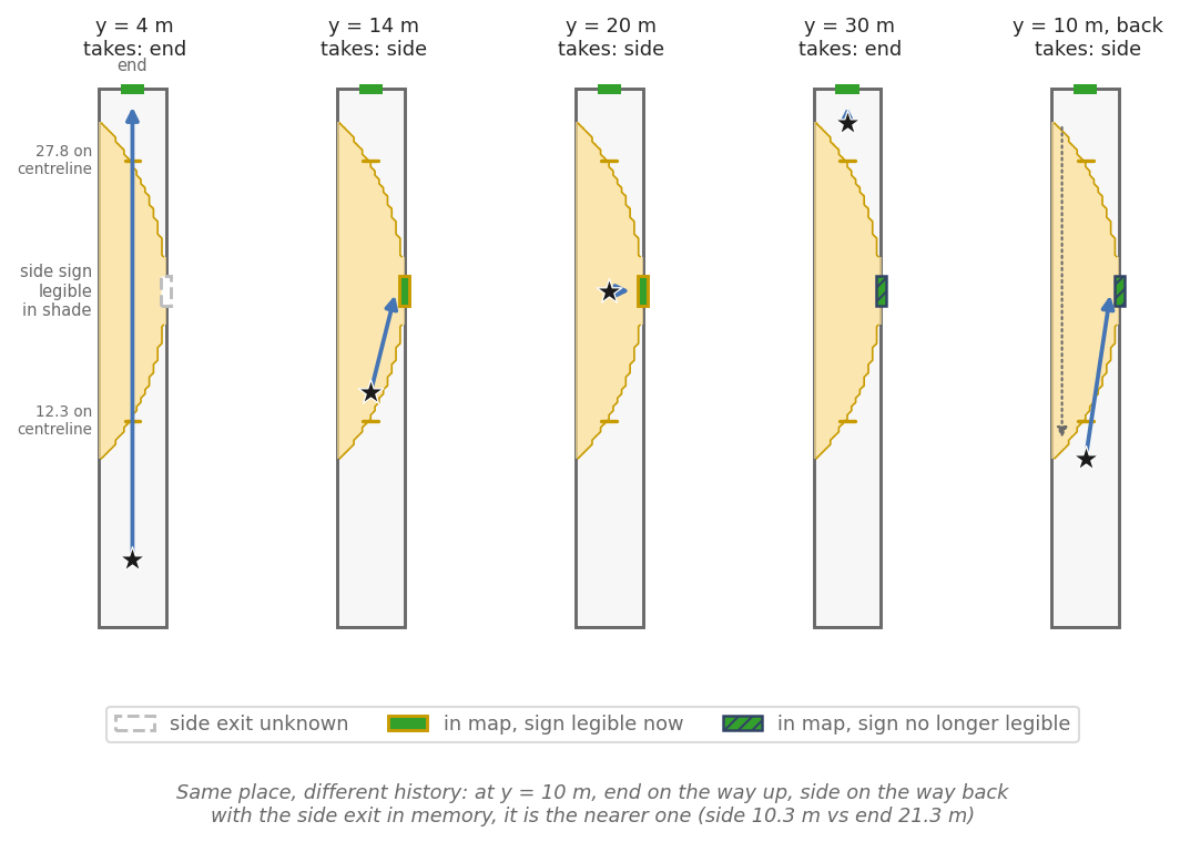
Figure 7. A corridor whose side-exit sign is legible only inside the shaded
region, y = 12.3–27.8 m on the centreline (gold ticks). One discovery agent is probed at a sequence of positions: northward,
then back south. These are probes, not a walk. Northward, the side exit is
learned inside the region and stays known beyond it, where the nearer end exit
ranks first. Back south, where the side sign cannot be read, the remembered
side exit is nearer and ranks first. Script: scripts/figures/map_memory.py.
The parameter split
Some parameters with the same name live in two places, and they do different
things. The walking-speed parameters (speed_law, alpha, beta,
min_speed_factor and visibility_factor_c) are fields of SmokeSpeedConfig.
run.py, the web GUI and the terminal UI build that object with its defaults,
so every run they start uses the Frantzich–Nilsson law with the FDS+Evac constants. Another law
or other coefficients require building the model in Python and passing it to
run_scenario().
The routing block of the scenario JSON accepts alpha, beta and
min_speed_factor with the same defaults. They only set the speed factor the
router uses to estimate travel time when it prices a route. Setting
routing.alpha changes which route an agent prefers, but not how fast it walks
in smoke. The same holds for speed itself: the router prices routes at its own
speed, routing.base_speed_m_per_s, not at the agent’s \(v_0\). The router
always uses the linear law, even when agents walk with the fridolf option. The
defaults are on the smoke-speed and
routing pages; see also
Limitations.
Notation
This table is the shared notation for the Concepts, Fundamentals and Models pages. Defaults are on the Models pages.
| Symbol | Meaning | Unit | Code name |
|---|---|---|---|
| K | Extinction coefficient at a point (FDS SOOT EXTINCTION COEFFICIENT) | 1/m | extinction_per_m |
| \(\bar K\) | Mean extinction along an edge or a route | 1/m | k_avg, k_ave_route |
| S = C/K | Sighting distance (Jin); V in the code’s fridolf option | m | — |
| C | Visibility constant of a sign (Jin); reflective or light-emitting | - | visibility_factor_c, sign c |
| \(v_0\) | Unimpeded desired speed of an agent | m/s | v0 (distribution group) |
| f(K) | Smoke speed factor | - | speed_factor |
| \(\alpha\), \(\beta\) | Frantzich–Nilsson coefficients | m/s, m²/s | alpha, beta |
| \(f_{\min}\) | Floor of the smoke speed factor | - | min_speed_factor |
| FIC | Fractional irritant concentration (Purser; related to, but not the same as, ISO 13571 FEC) | - | fic |
| g(FIC) | Irritant speed factor | - | fic_min_factor, fic_alpha |
| FED | Fractional effective dose, toxic gases | - | fed |
| \(\mathrm{FED}_{\mathrm{heat}}\) | Fractional effective dose, convective heat | - | heat FED |
| \(D_i\), \(D_{\mathrm{heat},i}\) | Incapacitation threshold of agent i; log-normal in probabilistic mode | - | fed_threshold for both; heat_fed_threshold overrides the heat one |
| T | Gas temperature | °C | TEMPERATURE slice |
| \(L_k\) | Walkable distance still to go on route k | m | effective_length |
| \(\tau_k = \bar K_k L_k\) | Optical depth along route k | - | tau_route |
| \(\tau_{\max}\) | Refusal budget for \(\tau\) | - | tau_max |
| \(\Delta s\) | Spacing of smoke samples where the field has no grid or the line leaves every FDS subslice, and of the walk-dose FED rate | m | sampling_step_m |
| \(\alpha_s\) | Bearing of a sign, degrees clockwise from north | ° | sign alpha |
The same code name alpha is used for the Frantzich–Nilsson coefficient, for
the irritant slope fic_alpha and for the sign bearing; the table keeps them
apart. In FDS+Evac, \(\tau\) is the relaxation time of the movement model. On
these pages \(\tau\) is always the dimensionless optical depth. “Gate” is used
in two senses only: the exposure gate (the route-cost gate) that refuses a
route, and sight gating, which decides whether a sign is legible and so what
enters the cognitive map. The dose does not gate anything; it stops the agent.
Further reading
- The talk: slides, Visibility Seminar 2026, University of Wuppertal, 25 September 2026.
- Fundamentals: the published laws, with their sources.
- Model pages: smoke speed, FED, routing, wayfinding, and verification.
- Limitations: what is not modelled, and which parameters are library-level.