When can we trust a crowd simulation? Lessons from a road paradox
Crowd simulations are used to plan stations, stadiums and evacuations. A simulation can reproduce empirical data and pass test cases that guidelines prescribe, which supports a particular claim. However, using the model for another geometry, another population or a decision about safety needs further evidence, and it is often unclear how much. In our own work, a model that matched a bottleneck experiment mostly within ten percent let people through an unguided entrance at more than twice the measured rate (section 6).
What a model explains and what it leaves open can be studied with a simple model: the Braess paradox, introduced in 1968 by the mathematician Dietrich Braess. Braess showed in a simple network model that a new road can make every driver slower (Braess 1968; English translation Braess et al. 2005). A good explanation of such a result makes specific consequences follow from explicit assumptions. Tests then show how far those consequences hold outside the model.
1. A road that makes everyone slower
Take a small road network with four nodes: Start, A, B and Goal. Two routes lead from Start to Goal, an upper one via A and a lower one via B. Each route has one narrow road, where the travel time is \(n\) minutes if \(n\) drivers use it, and one wide road without congestion, where the travel time is constant (\(C\) minutes). As in normal life, every driver wants to reach the goal as fast as possible. (Who wouldn’t?)
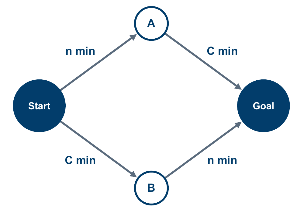
The network. On the narrow roads the travel time grows with the number of drivers n; on the wide roads it is a constant C.
Let’s consider 15 drivers and \(C = 17\). The model specifies an equilibrium: a split of the drivers in which nobody can arrive sooner by switching route alone. With 7 drivers on the upper route and 8 on the lower one, the upper route takes 24 minutes and the lower one 25. A driver who switches from the lower to the upper route would then also need 25 minutes. This state is a Nash equilibrium.1
Now imagine the city decides to build a shortcut from A to B with a travel time of zero. In this situation, drivers have three different routes: upper, lower, and Start → A → B → Goal.
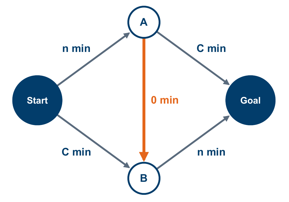
The same network with a shortcut from A to B that takes no time at all.
Start from the old split, 7 drivers on the upper route and 8 on the lower one. One driver from the upper route tries the shortcut. The first narrow road still carries 7 drivers, the second now carries 9. This driver needs \(7 + 0 + 9 = 16\) minutes instead of 24, because the 17-minute wide road is replaced by a narrow road that takes 9 minutes. The driver gains 8 minutes, and everyone on the second narrow road loses one.
The model does not say how drivers get to the new equilibrium. If they switch one at a time whenever switching shortens their own trip, they keep moving to the shortcut as long as both narrow roads together cost less than one narrow and one wide road. So the drivers move over, and the narrow roads fill up. In the end all 15 use the shortcut, and each needs \(15 + 0 + 15 = 30\) minutes. A driver who goes back to the upper route alone needs \(15 + 17 = 32\) minutes, more than 30. So nobody leaves the shortcut, although without it everyone would arrive sooner. This is again a Nash equilibrium, but a worse one. The old split of 7 and 8 would be better for everyone, but with the shortcut it is no longer an equilibrium.
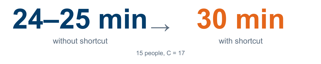
The two equilibria for 15 drivers and C = 17: 24 to 25 minutes without the shortcut, 30 minutes with it.
Try it yourself. The game keeps \(C = N + 2\), so \(C\) changes with the number of drivers. Move the drivers between the routes, switch the shortcut on, and watch where the travel times settle. The box below the bars tells you whether anyone can still gain by switching.
Average over all drivers:
2. What explains the result?
Here are two possible explanations for the paradox.

Explanation A blames selfish drivers. Explanation B says which route is cheapest for each driver and how its load grows.
Explanation A sounds plausible but names no mechanism. “Selfish” could explain the opposite result as well, and A does not say under which conditions the paradox occurs. Explanation B says which roads fill up and why. B connects assumptions to consequences. We can change an assumption, for example the travel time of the shortcut, but then the model determines what follows, so B cannot be adjusted to fit any outcome. That is why B makes predictions: consequences calculated from the model; whether people behave this way is a question for section 4.
Unlike A, explanation B shows how the road acts. The shortcut adds a route, and the longer travel times arise because traffic redistributes onto the two narrow roads. The drivers react to each other: my route choice changes your travel time, your travel time changes your route choice, and that changes mine again. Such feedback is the rule in traffic and pedestrian dynamics.
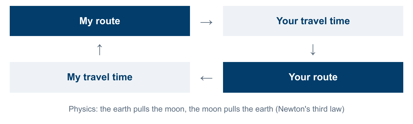
The feedback loop in the route game: my route changes your travel time, your travel time changes your route, and your route changes my travel time.
3. What the model claims
Each driver chooses the fastest route, and the result is worse for all. That is what the model predicts. But the model assumes that travel time grows with the number of vehicles, that everyone chooses the fastest route and that the new road takes no time.
The road network is a model: a simplified image of reality. A lot has been left out of it. For instance:
- People: drivers who do not choose the fastest route.
- Traffic: traffic lights, junctions, queues.
- Roads: lengths, widths, capacities.
- Travel time: where the rule of \(n\) minutes comes from; behind it lies the fundamental diagram.
- Time: how route choices change from day to day, and whether traffic settles into the equilibrium at all; the model only states the equilibrium.
- Information: how drivers learn the travel times; in the model everyone knows them.
A model does not have to contain every detail of reality, though. It has to capture the mechanisms that matter for the question, here the link between route choice, traffic load and travel time; the colour of the cars does not matter, and neither does their brand. With four nodes and five edges it explains something surprising. Box (1976) wrote: “Since all models are wrong the scientist must be alert to what is importantly wrong.” Whether we left out the right things is a question for validation (section 5).
Assumption, theory, hypothesis, prediction
- Assumption: “Drivers choose the route that is fastest for them.” This is an assumption about behaviour. It is assumed within the model; whether people behave this way is a separate, testable question. It is not a theory. The model consists of this assumption together with the network, the number of drivers and the travel-time rules of the roads.
- Theory: a coherent set of statements built on such assumptions, from which consequences can be derived. Here it is the equilibrium theory of route choice after Wardrop (1952). Its first principle: in equilibrium the travel times on all used routes are equal, and no unused route is faster.
- Hypothesis: a proposed explanation that can be tested. For example: drivers respond to their own travel times in a way that concentrates traffic on the two narrow roads.
- Prediction: an observable consequence of the hypothesis under stated conditions, which can fail against data. For example: “If the shortcut in this network is closed, the mean travel time decreases.”
Following Popper, ask which observation would refute a prediction. If you cannot name one, the claim is not yet empirically testable.
An example of how a question becomes testable: “A bottleneck 3 m wide and 1 m long, or 1 m wide and 3 m long: which is better?” As it stands, the question is too vague to answer. One has to fix the walking direction,2 the geometry, and what “better” means: higher flow, shorter evacuation time or lower density in front of the bottleneck. Only then does the question become testable. A prediction would add the expected answer, for example that the wider bottleneck gives the higher flow.
Verify or falsify?
Karl Popper (Logik der Forschung, 1934; Conjectures and Refutations, 1963, ch. 1) pointed out that general statements can never be proven conclusively, because nobody has seen all cases. A hundred cities in which a new road helped do not prove that new roads always help. One Braess case is enough to refute it, but only because the statement is universal (“always”). A single counterexample does not refute “mostly”.
In practice a refutation is rarely this clean. A prediction always rests on auxiliary assumptions about instruments, data and conditions. When a prediction fails, something in this group of assumptions is wrong, but the failure does not say which part (Duhem 1954, part II, ch. 6); it may be an auxiliary assumption instead of the theory. This is known as the Duhem–Quine problem, and it is one reason why a single surprising observation rarely settles a dispute.
One warning about words: in simulation, “verification” means something else, namely checking the program (section 5).
Three levels have to be kept apart: the model, people playing the route game, and real traffic. The mathematical result is knowledge about the model. Whether real traffic behaves like either is a further empirical question. If players and model differ, the next step is to find out which modelling assumptions or experimental conditions account for the difference, or whether the game had not yet settled.
4. Testing competing explanations
Reports from Stuttgart in 1969 (Knödel 1969), New York in 1990 (Kolata 1990) and Seoul in 2003 to 2005 (Chung et al. 2012) are often cited for the paradox. They are observations after an intervention, not controlled experiments; Rapoport et al. (2009, p. 539) call them “sketchy and mostly anecdotal”. In a city many things change at once, and the observations alone do not show what caused the change.
A laboratory game can isolate the shortcut. Playing one version first can change behaviour in the second, so a clean design gives groups the two-route and the three-route game in both orders, keeps the number of people, the travel-time rules and the information the same, and runs each game for several rounds. Rapoport and colleagues (2009) ran this game with groups of students paid according to their travel costs. Reversing the order made no difference. In a network with the same structure as ours, the groups moved to the shortcut route, and their payoff fell sharply. This shows the effect of adding the shortcut for these players under these conditions. It is not yet evidence about real road networks. Whether the players reached the result through the feedback of section 2 is a separate question; it would need data on how route choices respond to travel-time information, for example the players’ own previous travel times.
A matching result can still have the wrong explanation. Around 1900 a horse, “Clever Hans”, tapped out correct answers to arithmetic questions in front of large audiences, and a commission found no trick in 1904. Two explanations fit the correct answers: Hans can do arithmetic, or Hans reads unconscious signals from the questioner. The psychologist Oskar Pfungst (1907) separated them by changing one condition at a time. When the questioner did not know the answer, or Hans could not see the questioner, the errors increased sharply. Pedestrian experiments can face the same kind of question. Instructions, demonstrations or other cues may shape what participants do, and a pattern that fits a proposed mechanism may also fit such conditions; a comparison that changes them can help separate the two, provided they predict different responses.
5. From a model to a simulation
The road network can be worked out by hand. A crowd in a building cannot; it needs numerical methods and software, for example the models on this site. If such software reproduces the analytical equilibrium of the Braess network exactly, it computes correctly for this test case. That is verification, not validation. The same holds for a pedestrian model: the program can implement a movement rule correctly, with a fundamental diagram, the relation between density and flow, taken from experiments, and the rule can still fail to predict how these people move in this building. People may choose exits differently than assumed, and queues, differences in information or changes in motivation may be missing.
The tempting conclusion is: “The input models are validated and the software passes all tests, so the simulation is realistic.” Two questions have to be asked separately: did we implement the model correctly, and did we choose the right model?
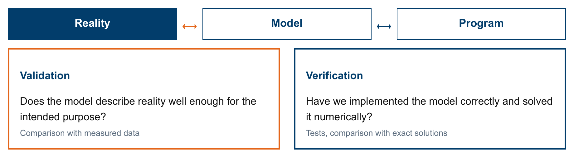
Verification compares the program with the model; validation compares the model with reality.
- Verification: does the program compute what the model says? Has the model been implemented correctly and solved numerically? This is checked with tests and comparisons with exact solutions, looking for errors in code and numerics.
- Validation: does the model describe reality well enough for its intended purpose? This is checked against measured data. A model is always valid for a purpose, never absolutely.
Roache (1998), following Boehm and Blottner, put it briefly: verification means solving the equations right, validation means solving the right equations.
6. How far does a successful model travel?
A good fit in one situation does not show that a model transfers to the next. We learned this the hard way. In a calibration study we fitted the Collision Free Speed Model to a bottleneck experiment. The result looked good: flow, density and speed in front of the opening matched mostly within ten percent, even at two widths we had left out of the fit. However, we ran the optimizer from two starting points, and it found two parameter sets that fit almost equally well. Their time gap and their repulsion (strength and range) differ by factors of two to four. So the good fit did not pin down the parameters. Hydrologists call this equifinality: different parameter sets, and even different models, can fit the same data acceptably well (Beven 2006). The bottleneck data cannot tell the two sets apart. Only a new situation can.
So in the second part we took the same parameters, without refitting, to two new situations: a half-metre gate and an entrance without guiding barriers. At the gate, one set stalls and the other lets 20 to 40 % more people through per second than were measured. At the entrance it got worse: every set let people through at more than twice the measured rate, about 1.3 against 0.57 persons per second. We suspect the model misses how people in such a crowd push to be first, but that is a hypothesis, not a result. Still we must say, a model calibrated for one situation was not valid for the next.
Claims about a model of human behaviour have to be specific to be tested. Often we read “our model reproduces human behaviour”, but such statements are simply too broad to be tested. A better statement would be, however, “our model estimates the flow through this exit, for this population and these conditions, with this uncertainty”, because such statement can be tested. Estimating the flow through a given exit is also a different task from predicting which exit people choose. The second rests on assumptions about behaviour that bottleneck flow measurements do not test.
7. What each method can show
So far we have drawn on four kinds of evidence: a model, laboratory experiments, reports from real cities and simulations. Each of them can show some things and not others.
Let’s start with simulations. Being able to run a simulation thousands of times does not make it more trustworthy than an experiment, or a field observation for that matter. Repeated runs of a stochastic model are still useful. They show when the mean evacuation time, its spread and the shape of the evacuation curve stop changing (Ronchi et al. 2014). However, they cannot show more than the model contains. If a model assumes that everyone knows all exits and takes the fastest route, a million runs with different random seeds will never produce a person who does not know the way. Models have to make such assumptions about behaviour, often without data to support them (Kuligowski 2013). Convergence tells us how precisely we know the model’s answer. Only data tell us whether that answer describes these people (section 5).
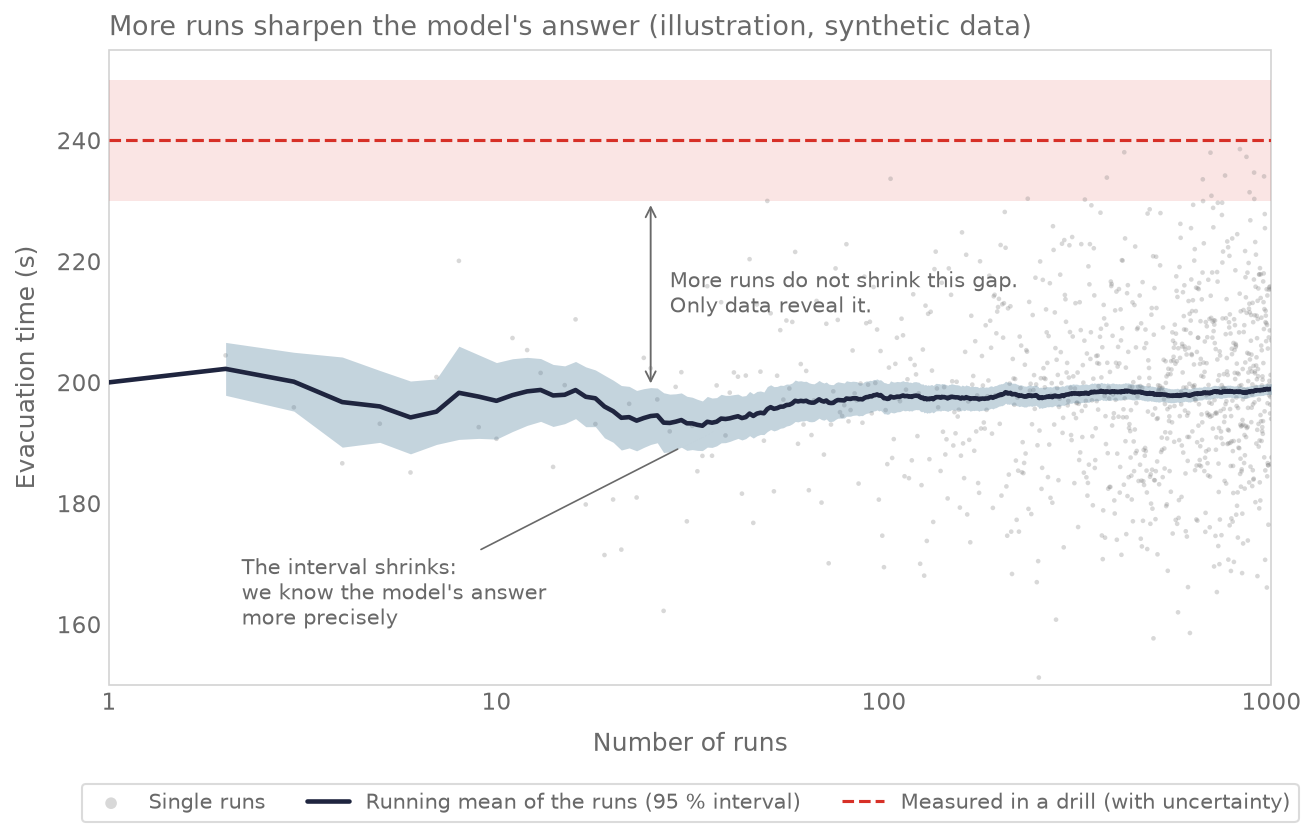
Illustration with synthetic data: the running mean of a stochastic model settles on the model’s own value as the runs accumulate, while a measured drill value stays where it is. (Script)
An experiment observes real people, but in one particular situation. A bottleneck experiment with instructed participants supports conclusions about movement under those instructions, densities and geometries. Whether they hold for another population, a different motivation or an emergency is another matter. Field observations have the opposite problem. They are closer to the real situation, but many factors vary at once, and being natural does not make them valid (Haghani 2023).
So each method is better at checking some parts of an explanation than others. Experiments are good at isolating a mechanism, observations at checking whether it transfers, and simulations at working out the consequences under conditions that we cannot test directly. They help each other because their weaknesses differ. Two sources with the same weakness can both add evidence, but neither can fix that weakness.
In discussions we often hear criticism of models, experiments and field observations that stays general: “models are just models”, “people don’t behave like that”, “experiments are not reality”. Each of these points to a real problem, but none says which conclusion is affected. With the terms of this essay we can turn them into questions that can be checked:
| Objection | Question to ask |
|---|---|
| “Models are just models.” | Which simplification could change the result we are using? |
| “People don’t behave like that.” | Which behaviour is missing, for which people and situation, and which prediction does it affect? |
| “Experiments are not reality.” | Which findings carry over to the target situation, and which depend on the experimental setting? |
| “Field observations are too messy.” | What can be measured reliably, and which influences can be told apart? |
| “We ran thousands of simulations.” | Which uncertainty did the runs reduce, and which assumptions stayed untested? |
A useful criticism names what is missing and says why it matters. For example: “The model does not include groups who wait for each other. This matters here, because the predicted benefit of the second exit depends on people spreading out independently.” Such a criticism can be checked, and it may be strong enough to rule out one particular use of the model.
8. What passing a standard establishes
Guidelines such as RiMEA, the German guideline for microscopic evacuation analyses, list test cases for simulation software. We use them ourselves, and they are useful: they catch errors and make results easier to compare. However, we often see their results stretched. “The software passes the RiMEA tests” becomes “the software is validated”, then “the results of this project are reliable” and finally “this design is safe”. Each step is a new claim and needs its own evidence. For most of its tests RiMEA does not even set pass limits (RiMEA 2025, Annex 1, A 2). The first test, for example, only checks that a person with a given walking speed crosses a corridor in the expected time. Whether that speed fits the people in the building, or whether they find the exits, the test does not say, and it was never meant to.
RiMEA itself warns about this. Its preamble calls a simulation “an idealized case” in which people move as the user specifies. It also states that there are not enough reliable data from evacuation drills for a thorough quantitative comparison, and that until such data exist, its other tests are sufficient (Annex 1, A 5). This sentence was translated from the IMO guidelines for passenger ships (IMO 2002). It has not changed since, neither in later IMO versions (IMO 2016) nor in RiMEA. In the meantime, laboratory data have appeared, and RiMEA now uses some of them.
IMO, RiMEA, the NIST report (Ronchi et al. 2013) and ISO 20414 share many tests, and most of them come from the same IMO list. So passing the same inherited test under several standards counts once.
RiMEA’s later tests compare models with laboratory data, mostly for trends or the spread of the data, and the user may change the parameters. Once software is tuned to pass a test, passing it tells us less about anything outside the test (Goodhart 1984; Strathern 1997). ISO 20414 (2020) asks for more: the field of application must be stated, a validation against one data set does not automatically carry over to other scenarios, and validation runs must also use default or generally representative settings, not only settings tuned to the data.
We think the tests themselves should be tested. We need to know which errors that would change a safety conclusion they can reveal, and which wrong predictions still pass them. That applies to our own software too. Passing a standard is one part of the argument for trusting a simulation. The rest has to come from evidence about the people, the building and the purpose of the simulation.
A note on standards
9. Using an explanation to make a decision
For practical projects the question becomes: what evidence is enough for this model to support this decision? A claim that a layout is safer needs a safety criterion, for example that everyone is out before conditions become untenable (ASET > RSET); a layout can be faster on average and worse for the last people out. Sometimes the answer is that the evidence does not support the proposed safety claim.
Suppose a well-tested model predicts that a second exit reduces the mean evacuation time of a hall. The prediction alone does not decide whether to build it. The exit may help most people and do little for the last ones out, and space, costs and everyday use count as well. Weighing them requires stating what we want to achieve. Science can say what is likely to happen under each option; which outcome to prefer is a decision about goals. Values also enter the science itself, for example when deciding how much evidence is enough to accept a claim, given the consequences of being wrong (Douglas 2009, ch. 5).
When can we trust a crowd simulation?
A good explanation names a mechanism that turns explicit assumptions into specific consequences. It cannot be adjusted to fit any outcome, so a test can show it wrong. In the road network this is easy to check, because every assumption is visible. A crowd simulation makes the same kind of claim with many more assumptions, and the evidence for it comes in parts.
Our calibrated model reproduced a bottleneck experiment mostly within ten percent, including two widths left out of the fit. That supports predictions of flow, density and speed under the tested conditions. Using it elsewhere needs an argument about which changes matter: two parameter sets that fit equally well behaved differently at a half-metre gate, and every set let people through an unguided entrance at more than twice the measured rate. The RiMEA tests give evidence about the quantities and behaviours they examine, under their test conditions and often without pass limits; they do not establish that a model suits a particular building or population. Trusting a simulation for a decision means stating the claim it is used for and checking that the evidence covers that claim.
The same questions apply to any scientific explanation or model-based claim, in a newspaper, a report or one’s own thesis:
- What exactly is explained, and what is the mechanism?
- Could the explanation be changed at will and still “explain” the same thing?
- Which observation would refute it?
- What evidence separates the explanation from plausible alternatives: a controlled comparison, independent observations that test predictions the alternatives get wrong, or only a sequence in time?
- Was a model checked against reality, and for which purpose is it valid?
Further reading
- David Deutsch, The Beginning of Infinity (2011), chapter 1, “The Reach of Explanations”. A shorter text by him: “Why It’s Good To Be Wrong”, Nautilus, 23 May 2013.
- Karl Popper, Conjectures and Refutations (1963), chapter 1, “Science: Conjectures and Refutations”.
- Naomi Oreskes, Why Trust Science? (2019).
- Peter Godfrey-Smith, Theory and Reality: An Introduction to the Philosophy of Science (2nd edition, University of Chicago Press, 2021), an introduction to the philosophy of science that compares several views.
Further material
References
- AIAA (1998): Guide for the Verification and Validation of Computational Fluid Dynamics Simulations. AIAA G-077-1998.
- Beven, K. (2006): A manifesto for the equifinality thesis. Journal of Hydrology 320(1–2), 18–36. doi:10.1016/j.jhydrol.2005.07.007.
- Box, G. E. P. (1976): Science and Statistics. Journal of the American Statistical Association 71(356), 791–799. doi:10.1080/01621459.1976.10480949.
- Braess, D. (1968): Über ein Paradoxon aus der Verkehrsplanung. Unternehmensforschung 12, 258–268.
- Braess, D., Nagurney, A., Wakolbinger, T. (2005): On a Paradox of Traffic Planning. Transportation Science 39(4), 446–450.
- Chung, J.-H., Hwang, K. Y., Bae, Y. K. (2012): The loss of road capacity and self-compliance: Lessons from the Cheonggyecheon stream restoration. Transport Policy 21, 165–178.
- Deutsch, D. (2011): The Beginning of Infinity: Explanations That Transform the World. London: Allen Lane.
- Douglas, H. E. (2009): Science, Policy, and the Value-Free Ideal. Pittsburgh: University of Pittsburgh Press.
- Duhem, P. (1954): The Aim and Structure of Physical Theory. Translated by P. P. Wiener. Princeton: Princeton University Press.
- Goodhart, C. A. E. (1984): Problems of monetary management: the U.K. experience. In: Monetary Theory and Practice: The UK Experience. London: Macmillan, 91–121. doi:10.1007/978-1-349-17295-5_4.
- Haghani, M. (2023): The notion of validity in experimental crowd dynamics. International Journal of Disaster Risk Reduction 93, 103750.
- IMO (2002): Interim Guidelines for Evacuation Analyses for New and Existing Passenger Ships. MSC/Circ.1033. London: International Maritime Organization.
- IMO (2016): Revised Guidelines on Evacuation Analysis for New and Existing Passenger Ships. MSC.1/Circ.1533. London: International Maritime Organization.
- ISO/TR 13387-8 (1999): Fire safety engineering — Part 8: Life safety — Occupant behaviour, location and condition. Geneva: ISO (withdrawn).
- ISO 20414 (2020): Fire safety engineering — Verification and validation protocol for building fire evacuation models. Geneva: ISO.
- Knödel, W. (1969): Graphentheoretische Methoden und ihre Anwendungen. Berlin: Springer.
- Kolata, G. (1990): What if They Closed 42d Street and Nobody Noticed? New York Times, 25 December 1990. Free summary: “42nd Street: Braess’s Paradox”, Cornell course blog Networks, 2016.
- Kuligowski, E. (2013): Predicting Human Behavior During Fires. Fire Technology 49(1), 101–120.
- Liddle, J., Seyfried, A., Klingsch, W., Rupprecht, T., Schadschneider, A., Winkens, A. (2009): An Experimental Study of Pedestrian Congestions: Influence of Bottleneck Width and Length. arXiv:0911.4350.
- Liddle, J., Seyfried, A., Steffen, B., Klingsch, W., Rupprecht, T., Winkens, A., Boltes, M. (2022): Microscopic insights into pedestrian motion through a bottleneck, resolving spatial and temporal variations. Collective Dynamics 7, A139, 1–23. doi:10.17815/CD.2022.139.
- Pfungst, O. (1907): Das Pferd des Herrn von Osten (Der Kluge Hans). Leipzig: Barth.
- Popper, K. (1934): Logik der Forschung. Wien: Springer.
- Popper, K. (1963): Conjectures and Refutations: The Growth of Scientific Knowledge. London: Routledge & Kegan Paul.
- Rapoport, A., Kugler, T., Dugar, S., Gisches, E. J. (2009): Choice of routes in congested traffic networks: Experimental tests of the Braess Paradox. Games and Economic Behavior 65(2), 538–571.
- RiMEA (2025): Richtlinie für Mikroskopische Entfluchtungsanalysen, version 4.1.1.
- Roache, P. J. (1998): Verification of codes and calculations. AIAA Journal 36(5), 696–702.
- Ronchi, E., Kuligowski, E. D., Reneke, P. A., Peacock, R. D., Nilsson, D. (2013): The Process of Verification and Validation of Building Fire Evacuation Models. NIST Technical Note 1822.
- Ronchi, E., Reneke, P. A., Peacock, R. D. (2014): A method for the analysis of behavioural uncertainty in evacuation modelling. Fire Technology 50(6), 1545–1571.
- Strathern, M. (1997): ‘Improving ratings’: audit in the British University system. European Review 5(3), 305–321.
- Wardrop, J. G. (1952): Some Theoretical Aspects of Road Traffic Research. Proceedings of the Institution of Civil Engineers Part II 1(3).
Disclosure: The author’s group develops JuPedSim, simulation software to which such tests apply. Some of the laboratory data that RiMEA uses in its tests, and the bottleneck studies cited above (Liddle et al. 2009, 2022), come from Armin Seyfried and colleagues at Forschungszentrum Jülich, where the author works.
By: Mohcine Chraibi
Traffic research uses the related Wardrop equilibrium (Wardrop 1952): the travel times on all used routes are equal, and no unused route is faster. It is usually stated for so many drivers that a single one does not change the travel times. With 15 drivers, one driver changes a narrow road by a whole minute, so in a Nash equilibrium the used routes can differ by one minute, here 24 and 25. ↩︎
The width across the direction of walking matters most. In one experiment the length made little difference between 2 and 4 m, and only an opening a few centimetres deep let noticeably more people through (Liddle et al. 2009, 2022). ↩︎