Calibrating a pedestrian model against real data, part 2: where it stops
A calibration is only validated within the domain it was tested in. Part 1 ended with two parameter sets, A and B, that reproduce flow, density and speed at five bottleneck widths of 2.4 to 5.0 m mostly within ten percent, though neither passes the stated tolerance everywhere, and that disagree with each other on what the model gets wrong at the widest opening. The desired speed is fixed at the 1.55 m/s measured on the Hermes participants in every set below; carrying that value to other experiments is an assumption. The sets found along the way:
| parameter | default | set A | set B | set C | set D | joint |
|---|---|---|---|---|---|---|
| desired speed [m/s] | 1.2 | 1.55 | 1.55 | 1.55 | 1.55 | 1.55 |
| radius [m] | 0.20 | 0.13 | 0.15 | 0.124 | 0.101 | 0.115 |
| time gap [s] | 1.0 | 0.81 | 0.55 | 1.038 | 0.958 | 0.962 |
| neighbor repulsion strength | 8 | 2.1 | 9.4 | 9.01 | 1.70 | 8.62 |
| neighbor repulsion range [m] | 0.10 | 0.25 | 0.10 | 0.062 | 0.336 | 0.189 |
| wall repulsion strength | 5 | 5 (fixed) | 5 (fixed) | 2.96 | 1.39 | 4.69 |
| wall repulsion range [m] | 0.02 | 0.02 (fixed) | 0.02 (fixed) | 0.072 | 0.105 | 0.031 |
| fitted to | Hermes 2.4, 3.6, 5.0 m | Hermes 2.4, 3.6, 5.0 m | CrowdQueue h0 | CrowdQueue h0 | both |
Sets A and B, and sets C and D, are two optimizer starts on the same data. The tools, observables and tolerances are those of part 1: JuPedSim, PedPy on both experiment and simulation, Dakota’s surrogate-based optimizer, and a decision rule of 6 % on flow and 10 % on density and speed, chosen as calibration weights and adopted as tolerances after the fact.
Step 6 — a second experiment, and where the model stops
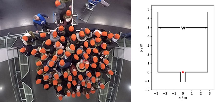
The CrowdQueue experiment, Wuppertal 2018: a run in the 5.6 m corridor seen from above, and the setup with the 0.5 m gate at the origin. Images: Pedestrian Dynamics Data Archive, Forschungszentrum Jülich.
The second open dataset is the CrowdQueue experiment from Wuppertal 2018 (Adrian et al. 2020): a crowd in front of an entrance again, but through a 0.5 m gate instead of a 2.4 to 5 m opening, in corridors from 1.2 to 5.6 m wide, with 11 to 75 participants and the motivation varied between runs. The archive files carry the full geometry and every trajectory, and each simulation is seeded from the data: agents in view at the first frame start there, and agents that enter the tracked corridor later are injected at the time and place of their first observation. Every tracked participant is simulated. An injection that finds its spot occupied is retried for 10 s and then dropped; this happened to one to four people in a few seeds of the two densest 1.2 m runs, and such a seed cannot count as emptied. Density and speed use the same window in experiment and simulation, the frames between the tenth and ninetieth percent of that run’s own crossings. Density is the time average over every frame; speed is averaged only over frames in which the area is occupied. Whether an observable is conditional on occupancy is part of its definition, and sparse runs expose the difference: averaging the zeros of empty frames had once reported 0.12 m/s instead of 0.56 m/s for the sparsest run. The flow is measured at a gate line and density and speed in a 2.2 m² upstream area, so the three values are not a flux identity and should not be forced to satisfy \(q=\rho v\).
Each run is simulated three times and every seed is shown, because averages hide the thing that matters here. A seed counts as emptied if every expected participant was injected and passed the gate within 120 s, twice the longest experiment. Otherwise it is not emptied, and if it also had an interval of 20 s or more without a crossing while agents remained, it counts as stalled. Flow is the slope of N(t) between the tenth and ninetieth percent of crossings for emptied runs; for runs that did not empty it is the number who passed divided by the time from the first crossing to the end of the run, which is lower by construction.
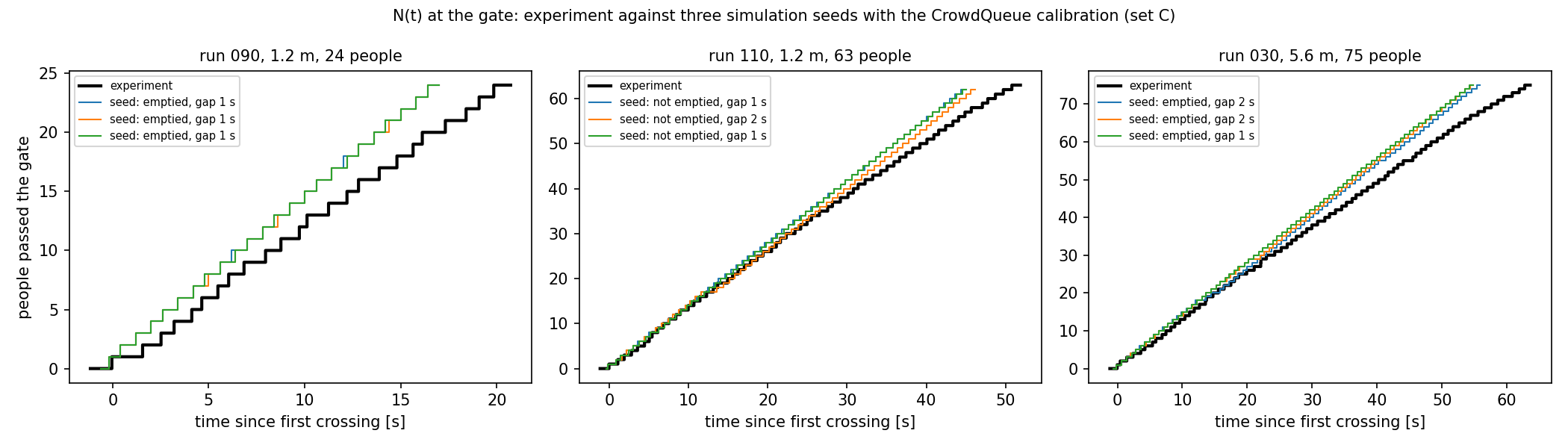
N(t) at the gate for three baseline runs, experiment against the three seeds of CrowdQueue set C. The simulated slopes are steeper than the measurements. In run 110 each seed passes 62 of 63 tracked participants because one late entrant could not be placed; none is classified as stalled.
The transfer test comes first: the two Hermes parameter sets applied to the 21 runs without refitting. Set A, the long time gap with weak long-range repulsion, stalls at the funnel in 46 of 63 seeds and empties 16. Set B, the short gap with strong short-range repulsion, empties 59 of 63 and stalls in none, but where it flows it overshoots the measured gate flow by 22 % on average in the baseline runs and by 37 % in the low-motivation runs. Of the two Hermes optima with near-equal residual norms on the wide bottleneck, one mostly stalls at a half-metre gate and the other passes it too fast. That is the practical meaning of the parameter compensation in part 1: sets with the same fit quality on one experiment behave differently on another.
Recalibrating on the seven baseline runs at 1.2, 3.4 and 5.6 m, with the wall parameters free because the 1.2 m corridors exercise them, was done from two optimizer starts, and again they disagree. Set C has a three-seed norm of 11.3 on its calibration runs and empties 59 of 63 seeds over all conditions. Set D has a norm of 16.2 and stalls in 14 seeds. Set C’s baseline flows are 12 % high on average, with individual runs from 2 % low to 30 % high. Its radius is 0.124 m; set D puts the radius almost at its 0.10 m lower bound. A second optimizer start changed both the inferred parameters and whether the narrow gate remained passable.
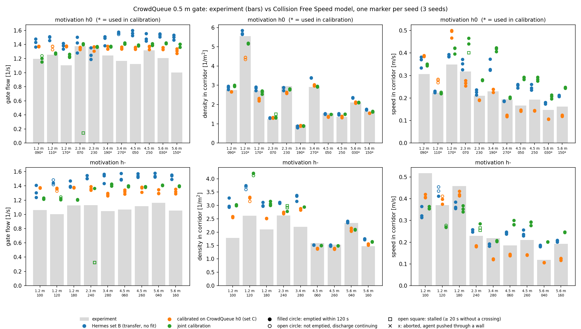
CrowdQueue: experiment (bars) against Hermes set B transferred without fitting (blue), the CrowdQueue calibration, set C (orange), and the joint calibration (green), one marker per seed, columns ordered by corridor width with the run number; asterisks mark the runs used in the calibration. Filled circle: the run emptied within 120 s; open circle: not emptied, discharge continuing; open square: stalled. Top: baseline motivation, bottom: low motivation.
The low-motivation runs show what a flow-only validation would miss. Between the baseline and the low-motivation condition the measured flow at the same gate is about 10 % lower; the model has no input for motivation, so with parameters fixed at the baseline calibration it predicts the same or a higher flow, and overshoots the low-motivation runs by 24 % on average. In the 1.2 m corridor with 24 people, set C gives a flow 29 % high, a front area 44 % denser than measured and people moving 21 % slower: throughput alone hides two compensating errors in the upstream state.
What static parameters can absorb
Can a different parameter set stand in for motivation? Freeing all seven parameters is a poor diagnostic because every interaction can compensate for every other one. We therefore freeze the five interaction parameters at set C and profile only desired speed v0 and time gap T, separately for the baseline condition h0 and the low-motivation condition h−. These profiles are fitted and evaluated on the same runs, with one-seed grids and Dakota runs that stopped at the iteration cap with their convergence criteria unmet. They are in-sample diagnostics, not a validated motivation model.
For h0, Dakota selects (v0, T) = (1.17 m/s, 0.79 s) with a three-seed norm of 9.19 over 33 residuals. For h− it selects (1.50, 1.73) with 11.74. Nearby low cells follow a diagonal valley in each grid, so the pair is constrained jointly more clearly than either coordinate is identified alone, the same degeneracy between desired speed and headway that Kretz et al. (2026) describe for the social force model. Neither profile point transfers to the other condition: the h0 point scores 15.65 on h− data and the h− point 13.95 on h0 data. The first profile had stopped at a bound of T = 1.2 s and appeared to show that no pair could represent h−; widening the box to 2.0 s removed that conclusion. A bound hit is a prompt for a sensitivity check, not a result.
The larger time gap reduces the residuals in this conditional slice. At the h− profile point, flow is within 13 % in every run and density within 11 % in seven of nine. It pays for that with speed: seven runs are 24 to 53 % too slow. Part of that residual is the observable rather than the model. The speed is a PedPy individual speed over a 0.4 s window, and people in the front area who move less than 10 cm in 2 s still register 0.09 to 0.13 m/s, a standing-frame floor that plausibly comes from head tracking and body sway. In the 4.5 and 5.6 m corridors the measured speeds of 0.12 to 0.21 m/s are within a factor of two of that floor, so a 10 % tolerance there is tighter than the observable resolves. We have not built an error model for it: the floor is an empirical warning, not a distribution, and we do not know how it varies with density or width or how it covaries with the density measurement. A post-hoc check with the radial speed towards the gate lowers the h− norm from 11.7 to 9.8 and leaves five runs more than two assumed standard deviations too slow. The static v0–T pair absorbs part of motivation, but it does not reproduce flow, density and speed together across corridor widths, and the speed residuals near the floor are poorly resolved.
The densities become tangible as head counts because the front area is 2.2 m². In the two 1.2 m pairs, the experiment averages 6.1 people for h0 against 3.9 for h− with 24 participants, and 12.2 against 5.8 with 63. With one common set C, simulation compresses those contrasts to 5.9 against 5.7 and 9.7 against 7.2. After the separate v0–T fits, the means become 5.6 against 5.0 and 12.3 against 5.6. The simulations replay each run’s observed initial positions and arrivals, so this is conditional evidence: it tests whether the model preserves the supplied positioning difference, not whether it generates that difference from motivation.
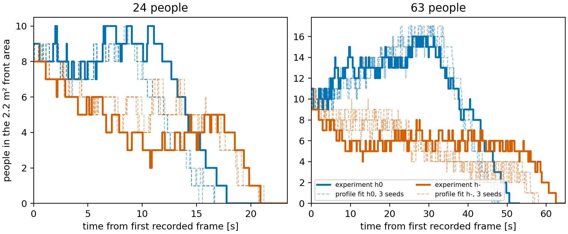
People inside the 2.2 m² area immediately upstream of the gate, experiment against three simulation seeds at the condition-specific v0–T profile points. The paired runs have the same corridor width and nominal population. Each simulation is conditioned on that run’s observed initial positions and arrivals; the figure is not a generative test of motivation.
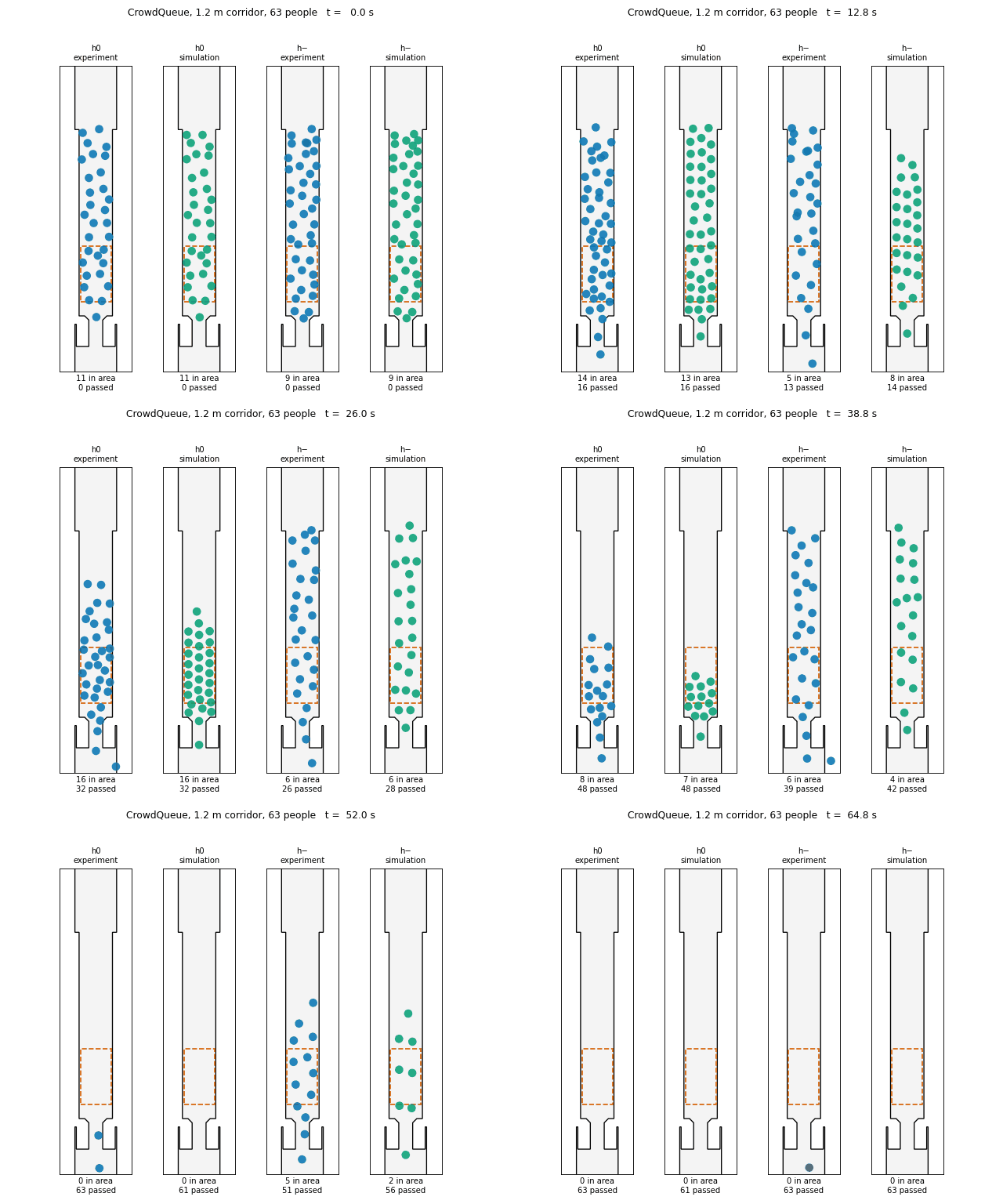
The two 63-person runs in the 1.2 m corridor, tracked experiment beside one simulation seed at the condition-specific v0–T profile point. The dashed rectangle is the front measurement area; the counts below each panel are the people inside it and the people who have passed the gate. Illustration only: the simulation starts from the observed positions, so the sparser low-motivation queue is partly inherited.
We also tested a spacing explanation by fixing v0 and T at the h0 profile point and varying radius and neighbor range. Its best point, radius 0.150 m and range 0.083 m, has a three-seed norm of 14.4, worse than the timing profile, and most of the surface is not a fit landscape but a stall cliff: from a neighbor range of 0.337 m upward all nine runs stall or fail at every radius, because radius and range govern both upstream separation and access through the same 0.5 m gate. This negative slice does not by itself identify the missing state variable.
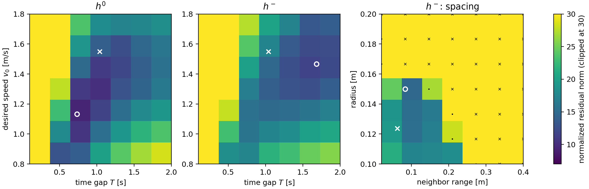
One-seed residual profiles with all unshown parameters fixed. Left and centre: desired speed v0 against time gap T for h0 and h−; right: radius against neighbor range for h− with v0 and T fixed at the h0 profile point. Open circles mark grid minima and white crosses the set-C coordinates. On the spacing panel, black dots mark grid points with some stalled or failed runs and black crosses points where all nine were stalled or failed. The common colour scale is clipped at norm 30.
The one high-motivation run, 11 people through the 1.2 m corridor at 2.1 persons per second, gets its own sweep over the time gap. A time gap near 0.3 s reaches the measured flow; there the density is about three times the measurement and the speed 30 % low. This condition has one usable run, so the sweep is a diagnostic, not a calibration.
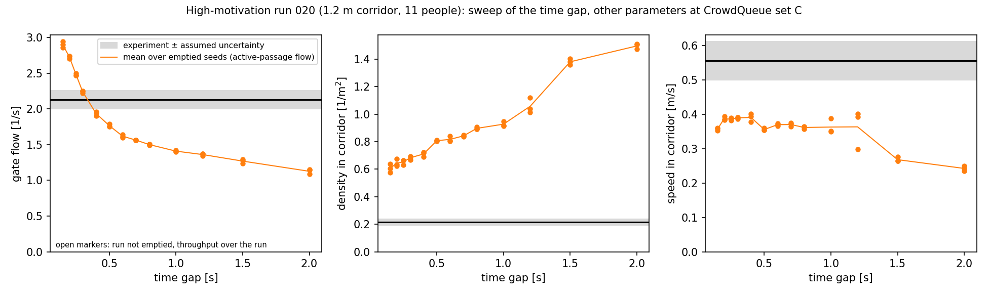
The high-motivation run: flow, density and occupied-frame speed in the corridor against the time gap, all other parameters at set C, three seeds per point shown individually. Filled markers and the line: runs that emptied. Grey band: the measured value with the uncertainty assumed in the calibration weights.
With the stated tolerance, recalibration on CrowdQueue makes passage reliable without bringing every observable within tolerance, and parameter sets that fit the wide bottleneck equally well behave very differently at the narrow gate. Why the remaining discrepancies are there, whether the round body, the interaction rules or something else, these tests do not say.
Step 7 — a third experiment, without barriers
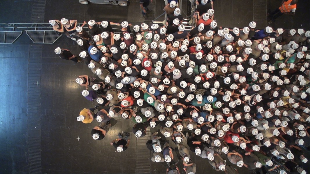
The BaSiGo entrance experiment, Düsseldorf 2013: the crowd in front of the unguided entrance, top right. Image: Pedestrian Dynamics Data Archive, Forschungszentrum Jülich.
The last test uses the BaSiGo entrance experiment from 2013 (Sieben et al. 2017): an entrance with two half-metre lanes and no guiding barriers, 319 people told that their favourite artist is playing and they want to be first in, 273 of them tracked. Nothing was fitted to it, and the comparison is a spatial profile rather than a number, the kind of comparison Liao et al. (2017) asked for, here conditional on the observed arrivals. The simulation injects each of the 273 tracked agents at the time and place where the data first see them. The 46 participants who were never tracked are absent, so the simulated crowd is about 15 % smaller than the real one, which changes the interactions in ways we did not quantify.
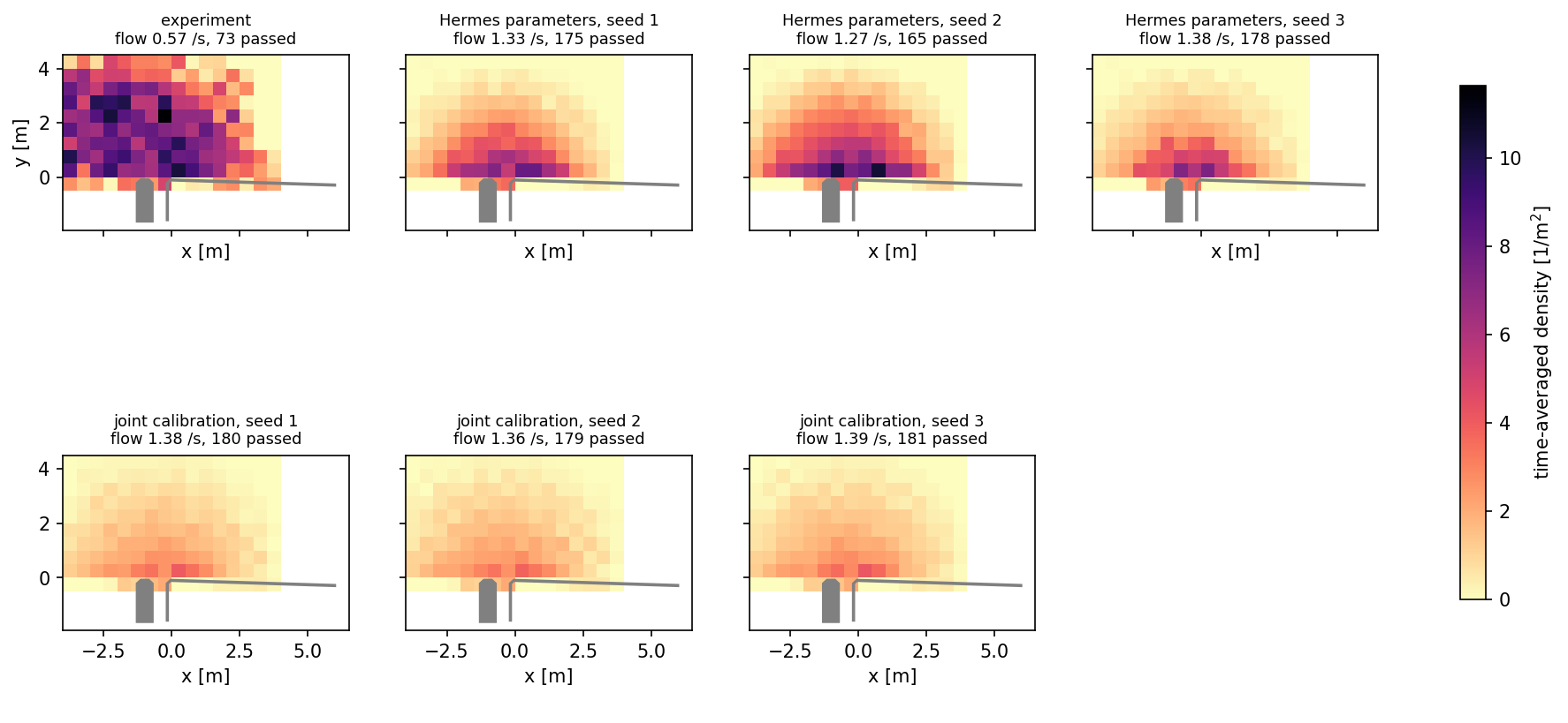
Time-averaged density in front of the entrance, 20 to 110 s into the run, on a 0.5 m grid: the experiment and each simulation seed separately, with its entrance flow over the same window and the number of people who passed within the 120 s run. Grey: the entrance barriers. Pale yellow is zero density; white lies outside the mapped grid.
Hermes set A produces a semicircle, but the wrong one. Its density is concentrated at the entrance and falls off regularly, with peaks around 6 per square metre; the measured crowd is dense to 10 per square metre over a region that extends two to three metres upstream and is visibly asymmetric, heavier to the left of the entrance. The model drains the crowd at 1.3 persons per second where the people, pushing to be first, achieved 0.57; the joint parameters give 1.36 to 1.39 persons per second, with the same regular shape. What the model lacks is a hypothesis, not a finding of this figure: we suspect the pressure of a crowd that wants to be first, and the shoulder rotation that gets real people through half a metre. The maps only show that the shape, the extent and the flow are all wrong, in the same direction for both parameter sets.
The joint calibration
The last set in the table comes from one Dakota run over both experiments: the three Hermes calibration widths and the seven CrowdQueue baseline runs, 30 residuals in all, each divided by its assumed uncertainty and entering with equal weight, so CrowdQueue carries about 70 % of the objective by count. One seed per run, one optimizer start, efficient_global with at most 40 iterations; both stopping criteria were met after 17. The result is compared with the specialists on post-hoc residual norms from stored seed means and on how many CrowdQueue seeds empty:
| parameter set | Hermes norm (9 residuals) | CrowdQueue norm (21 residuals) | CrowdQueue seeds emptied / stalled / otherwise not emptied |
|---|---|---|---|
| Hermes set A | 2.7 | 30.0 | 16 / 46 / 1 |
| Hermes set B | 2.4 | 14.9 | 59 / 0 / 4 |
| CrowdQueue set C | 11.3 | 59 / 0 / 4 | |
| CrowdQueue set D | 16.2 | 47 / 14 / 2 | |
| joint | 6.2 | 13.6 | 57 / 3 / 3 |
The joint point is worse than the relevant specialist in both experiments: 6.2 against 2.4 to 2.7 on Hermes, and 13.6 against 11.3 on CrowdQueue. The single search found no parameter set that meets the stated tolerances in both experiments. Whether a better compromise exists elsewhere in the parameter space, one start cannot say.
What happened to the calibrated model
It is worth being plain about it. After Hermes we had two parameter sets that reproduced five bottleneck widths mostly within ten percent, neither passing the tolerance everywhere. At a half-metre gate one of them stalled in 46 of 63 seeds and the other was 20 to 40 % too fast. The set calibrated on the gate passes it in every seed in which everyone could be placed, with flows 12 % high on average. Separate timing parameters reproduce much of the front occupancy contrast between baseline and low motivation, in-sample and conditioned on the observed positions, but not the speed. At the unguided entrance every set tested drains the crowd two to three times faster than the people did. The one parameter that was actually measured, the free speed, was the one the first optimizer run most wanted to change.
None of this is a verdict on the Collision Free Speed model in particular. It is what cross-regime transfer testing looks like, as opposed to a fit within one regime. Other pedestrian models with a handful of scalar parameters and round agents may show similar limits, but this note tests one model on three datasets and claims no more.
Lessons
- A calibration is a statement about a regime, not about a model. Parameters fitted to wide bottlenecks are parameters for wide bottlenecks. Using them for a turnstile, a narrow door or an unguided entrance is an extrapolation, and here it was off not by percent but by clogging or not clogging. Report the experiments a parameter set was fitted to and tested on; without that, “calibrated” is not information.
- State the purpose, then pick the observables. Flow alone would have passed a model with the wrong density, as it did in 2014. Analyse experiment and simulation with the same code, so the observables are defined once.
- Measured quantities are data, not fitting variables. Fixing the free speed at its measured value removed one unphysical value from the fit. It did not make the remaining parameters physical, and the value itself was measured on one experiment’s participants and assumed for the others.
- Run the optimizer more than once. Every calibration in this note that was started twice gave two different parameter sets. Multiple starts are a robustness check, not a map of the landscape, and a set reported without one is a sample.
- Screen before you calibrate. The Morris run cost 160 evaluations, removed two of seven parameters, and mapped a region where the model fails outright. Use sensitivity analysis for the grouping of parameters unless you have paid for converged indices.
- Measure an observable’s noise floor before you weight it. People standing still register about 0.1 m/s with the speed definition we calibrated against, and the wide-corridor speeds are within a factor of two of that. Estimate the floor first, and do not read residuals near it as well resolved.
- A fitted parameter shift is not a mechanism. The timing profiles absorb part of low motivation and the spacing slice develops a stall cliff. Both are useful diagnostics; neither says what motivation is. Keep parameter uncertainty and seed variability separate, and label as exploratory whatever was chosen after looking at the data.
- Audit the pipeline before you audit the model. Reviews of earlier drafts found late participants missing from simulations, unwritten final trajectory frames, a route around rather than through the gate, empty frames averaged as zero speed, and one script that ran set D while its output was discussed as set C. Each was plausible, produced numbers, and changed a conclusion. Each was corrected and every dependent result recomputed. The drivers now record an evaluation status file for every simulation, and the pipeline corrections section of the repository README lists each error and its fix, pinned to the commit this note was built from.
Several limitations remain open: one realization per condition, correlated observables, pragmatic weights, one optimizer start for the joint search, no time-step convergence study and no quantified observation error. The next useful work is not a uniquely calibrated parameter set but independent repetitions, more spatial and temporal observables, an explicit motivation state, a pre-specified uncertainty model and verification tests independent of the calibration data. Until then the conclusion is conditional: these scripts demonstrate a reproducible calibration and validation workflow and expose regime failures. They do not establish the validity of the model.
A note on open-source software
Sargent drew the cost of validation against the confidence it buys as a curve that rises steeply near the end. Everything in this study is about pushing that curve down. The trajectories are on a public archive with a DOI and the geometry attached, the model is open source and scriptable, the analysis library is the same one used on the experiment, and the calibration toolkit has been maintained by a national laboratory for 25 years. Anyone who thinks a remaining discrepancy is a model deficiency can test it this afternoon. And a validation that lives in a text file can be reviewed, which a sentence like “parameters were chosen according to the literature” never could.
References
- Adrian, J., Seyfried, A., Sieben, A. (2020). Crowds in front of bottlenecks at entrances from the perspective of physics and social psychology. Journal of the Royal Society Interface 17, 20190871. doi:10.1098/rsif.2019.0871.
- Kretz, T., Eckes, L., Knappik, L., Diz, J., Lipp, D., Müller, S. (2026). Using empirical travel time distributions for calibration of a model of pedestrian dynamics. EURO Journal on Transportation and Logistics 15, 100179. doi:10.1016/j.ejtl.2026.100179.
- Liao, W., Chraibi, M., Seyfried, A., Zhang, J., Zheng, X., Zhao, Y. (2014). Validation of FDS+Evac for pedestrian simulations in wide bottlenecks. IEEE ITSC 2014, 554–559. doi:10.1109/ITSC.2014.6957748.
- Liao, W., Zhang, J., Zheng, X., Zhao, Y. (2017). A generalized validation procedure for pedestrian models. Simulation Modelling Practice and Theory 77, 20–31. doi:10.1016/j.simpat.2017.05.002.
- Sargent, R. G. (1984). Simulation model validation. In: Simulation and Model-Based Methodologies: An Integrative View, Springer, 537–555.
- Sieben, A., Schumann, J., Seyfried, A. (2017). Collective phenomena in crowds — where pedestrian dynamics need social psychology. PLOS ONE 12(6), e0177328. doi:10.1371/journal.pone.0177328.
- Experiment data: Hermes bottleneck experiment, Düsseldorf 2009, doi:10.34735/ped.2009.6; CrowdQueue experiment, Wuppertal 2018, doi:10.34735/ped.2018.1; BaSiGo entrance experiment, Düsseldorf 2013, doi:10.34735/ped.2013.2. Dakota: Adams et al., Sandia National Laboratories, version 6.24.
Code
Driver scripts, Dakota input files, results and figures for every step: github.com/PedestrianDynamics/jupedsim-dakota-calibration
Software used in this study:
By: Mohcine Chraibi