Calibrating a pedestrian model against real data, part 3: default values for JuPedSim 2.0
Why new defaults
The current release of JuPedSim is 1.4.2. Version 2.0 is developed on the main branch of the repository and is not released yet. Parts 1 and 2 used 1.4.2. This part uses the main branch, i.e. the development version of 2.0 (see the end of the note for the commit). JuPedSim 2.0 renames its operational models (issue #1723). Models that reproduce a paper are frozen under the paper’s name. CollisionFreeSpeedModel is the one model that keeps improving, and it is the default. It is the model called CollisionFreeSpeedModelV2 in 1.4.2. Its default parameters, the same in both versions, were chosen by hand years ago (time gap 1 s, radius 0.2 m, neighbor repulsion strength 8 and range 0.1 m). Part 2 showed what such values are worth in another regime. Therefore, we asked which values a user should get when they choose nothing.
There was a second reason. A reader of Xu et al. (2019) asked why the model clogs in a 1.0 m bottleneck while the experiment does not. We reproduced Fig. 11 of that paper with the Collision Free Speed model in JuPedSim 1.4.2. With the time gap fitted to the flow, the model matches the experiment with an RMSE of 0.21 1/s. However, 4 of 10 runs at 1.0 m deadlock at the gap entrance, and on JuPedSim 2.0 the same parameters deadlock in 8 of 10 runs.
The mechanism, and one parameter against it
In every deadlocked run, the agents in the front row have zero spacing in their direction of motion. The crowd behind pushes them sideways against the wall next to the opening. Their direction is the sum of the desired direction and the repulsion from all neighbors within range, and the repulsion from behind dominates. The agents turn towards the wall, see a neighbor or a wall in their path, and stop. Since the speed of the model is a function of the spacing only, nothing restarts them.
The Generalized Centrifugal Force Model (Chraibi et al. 2010) weights a neighbor’s force by the cosine of its angle to the desired direction, and ignores neighbors behind. We added this vision factor to the direction rule of the Collision Free Speed model. With \(\mathbf{e}_0\) the desired direction and \(\mathbf{e}_{ij}\) the unit vector from agent \(i\) to neighbor \(j\), the repulsion of \(j\) is multiplied by
$$ w_{ij} = 1 - \lambda + \lambda \max(0,\, \mathbf{e}_0 \cdot \mathbf{e}_{ij}). $$\(\lambda = 0\) is the isotropic model, and \(\lambda = 1\) is the full vision factor. The parameter is called neighbor_repulsion_anisotropy. Its default was kept at 0 until the calibration decided on a value.
We tried a second remedy: tolerating a small overlap in the spacing. It turned deadlocks into clogs of up to 43 s, which is not better for a user, and we dropped it.
Moving to JuPedSim 2.0
We ported the drivers of part 1 and part 2 to the 2.0 interface. In 2.0, the walkable area is built as regions, the agents carry their parameters as a model state, and trajectories are written to HDF5. With the same parameters (set B of part 1, Hermes 2.4 m, one seed), the main branch gives a flow of 6.33 1/s and a density of 5.80 1/m², against 6.56 1/s and 5.60 1/m² on 1.4.2. The difference is within 4 %. Therefore, the new routing does not change this scenario noticeably.
However, two problems of 2.0 affected the work. First, one Hermes run takes 73 s on 2.0 and 5 s on 1.4.2. A profile attributes 99 % of the model time to the wall query, which uses exact geometric predicates and handles an exception on every lookup. Second, about 5 % of all runs aborted with the error path hit a wall, i.e. a step that would cross a wall. We counted these runs as failures. Both problems belong to the engine, not to the model, and are reported separately.
The objective
We kept the observables, weights and tolerances of part 1 and part 2. The residuals are flow, density and speed at Hermes 2.4, 3.6 and 5.0 m and at seven CrowdQueue runs with baseline motivation, each divided by 6 % (flow) or 10 % (density, speed) of the measured value. These are 30 residuals. The desired speed is fixed at the measured 1.55 m/s.
Part 2 showed that a stalled run can report observables that look fine. Therefore, we added a 31st residual: 5 for every run that stalls or fails. One stalled run costs 25 in the sum of squares, as much as one observable off by five tolerances. A run counts as stalled when nobody passes for 20 s. Each evaluation averages two seeds per scenario, i.e. 20 simulations, and takes 2.5 to 8 minutes on 12 cores.
We ran Dakota’s efficient global optimizer twice for each of \(\lambda = 0\) and \(\lambda = 1\), with six free parameters. Each study converged after 31 to 45 evaluations.
| study | best sum of squares | Hermes | CrowdQueue | stalled runs |
|---|---|---|---|---|
| \(\lambda = 0\), start 1 (set A) | 218 | 16 | 177 | 1 |
| \(\lambda = 0\), start 2 (set B) | 250 | 110 | 140 | 0 |
| \(\lambda = 1\), start 1 | 735 | 208 | 527 | 0 |
| \(\lambda = 1\), start 2 | 448 | 121 | 301 | 1 |
| joint set of part 2, JuPedSim 1.4.2 | 241 | 38 | 203 |
The isotropic model fits best, and the full vision factor fits CrowdQueue about twice as badly. As in part 1 and part 2, two starts on the same data end at different parameters.
Two seeds are a sample
We re-evaluated the best sets with five seeds, i.e. 50 simulations per set, see Fig. 1 (b). Set A, the best isotropic set, stalls in 13 of 50 runs, twelve of them at the CrowdQueue gate. Its sum of squares rises from 218 to 4569. The optimizer had chosen it on two lucky seeds. Set B stalls in 4 of 50.
The same sets with \(\lambda = 0.5\) stall in 0 and 1 of 50 runs, at a sum of squares of 318 and 328. With \(\lambda = 1\), they stall in 0 and 1 of 50 runs, but CrowdQueue fits worse (677 and 764). Therefore, we ran two more studies with \(\lambda = 0.5\) fixed and three seeds per evaluation. Their best sets, C and D, reach 250 and 261. With five seeds, set C has a sum of squares of 226 and no stalled run in 50. It is the only set in our tests that is below the joint set of part 2 (241) and does not stall.
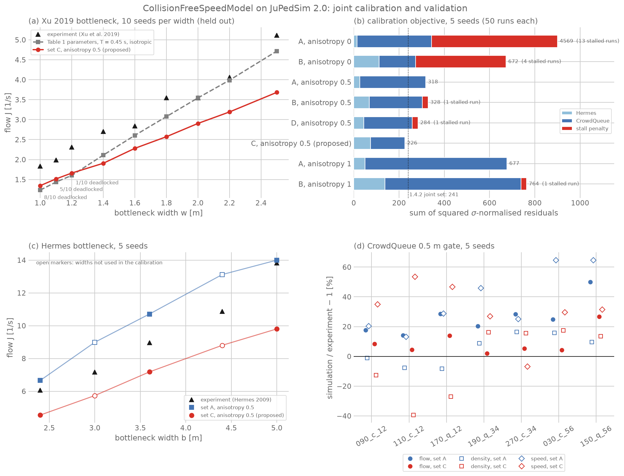
Fig. 1. (a) Flow in the bottleneck of Xu et al. (2019), not used in the calibration, 10 seeds per width. (b) Calibration objective of all candidate sets, re-evaluated with 5 seeds; red is the stall penalty, the bar of set A with \(\lambda = 0\) is cut at 900. (c) Hermes flow; open markers are widths not used in the calibration. (d) Relative error of flow, density and speed at the seven CrowdQueue runs.
The selected set
| parameter | current default | proposed (set C) |
|---|---|---|
| radius [m] | 0.20 | 0.155 |
| time gap [s] | 1.0 | 0.956 |
| neighbor repulsion strength | 8.0 | 2.83 |
| neighbor repulsion range [m] | 0.10 | 0.150 |
| wall repulsion strength | 5.0 | 5.95 |
| wall repulsion range [m] | 0.02 | 0.021 |
| neighbor repulsion anisotropy \(\lambda\) | 0 | 0.5 (fixed in the search) |
Set C is a compromise, and Fig. 1 shows where it pays. At the CrowdQueue gate, the flow is within 15 % in six of seven runs, see Fig. 1 (d). However, the speed in front of the gate is 27 to 53 % too high in six of seven runs. At the Hermes widths used in the fit, the flow is 20 to 29 % too low, see Fig. 1 (c). Set A with \(\lambda = 0.5\) fits Hermes better, but overestimates the gate flow by 14 to 49 %. We preferred the set that is closer at the narrow gate, since clogging and gate flow are where a wrong default misleads a user most.
Tests on data not used in the fit
Hermes 3.0 and 4.4 m. With five seeds, set C underestimates the flow by 3.3 and 3.2 tolerances, i.e. about 20 %, and the density by 1.7 and 2.1 tolerances. Set A with \(\lambda = 0.5\) overestimates the flow by 4.2 and 3.4 tolerances. Neither set meets the 6 % tolerance at the widths it was not fitted to. In 3 of 20 runs, one agent of 350 remained in a corner of the waiting area. We did not count this as clogging.
Xu et al. (2019), 1.0 to 2.5 m. With the desired speeds of that paper (normal, mean 1.34 m/s, standard deviation 0.26 m/s), set C does not deadlock in any of 90 runs, see Fig. 1 (a). The largest gap between two passages is 2.0 s. However, the flow is 18 to 29 % below the experiment from 1.4 m on. This agrees with the underestimation at Hermes, and the lower desired speed adds to it.
Current and proposed defaults
In this section, we compare what a user gets without setting any parameter. Both sets run in the bottleneck of Xu et al. (2019) with every agent at the default desired speed of 1.2 m/s, 10 seeds per width, see Fig. 2.
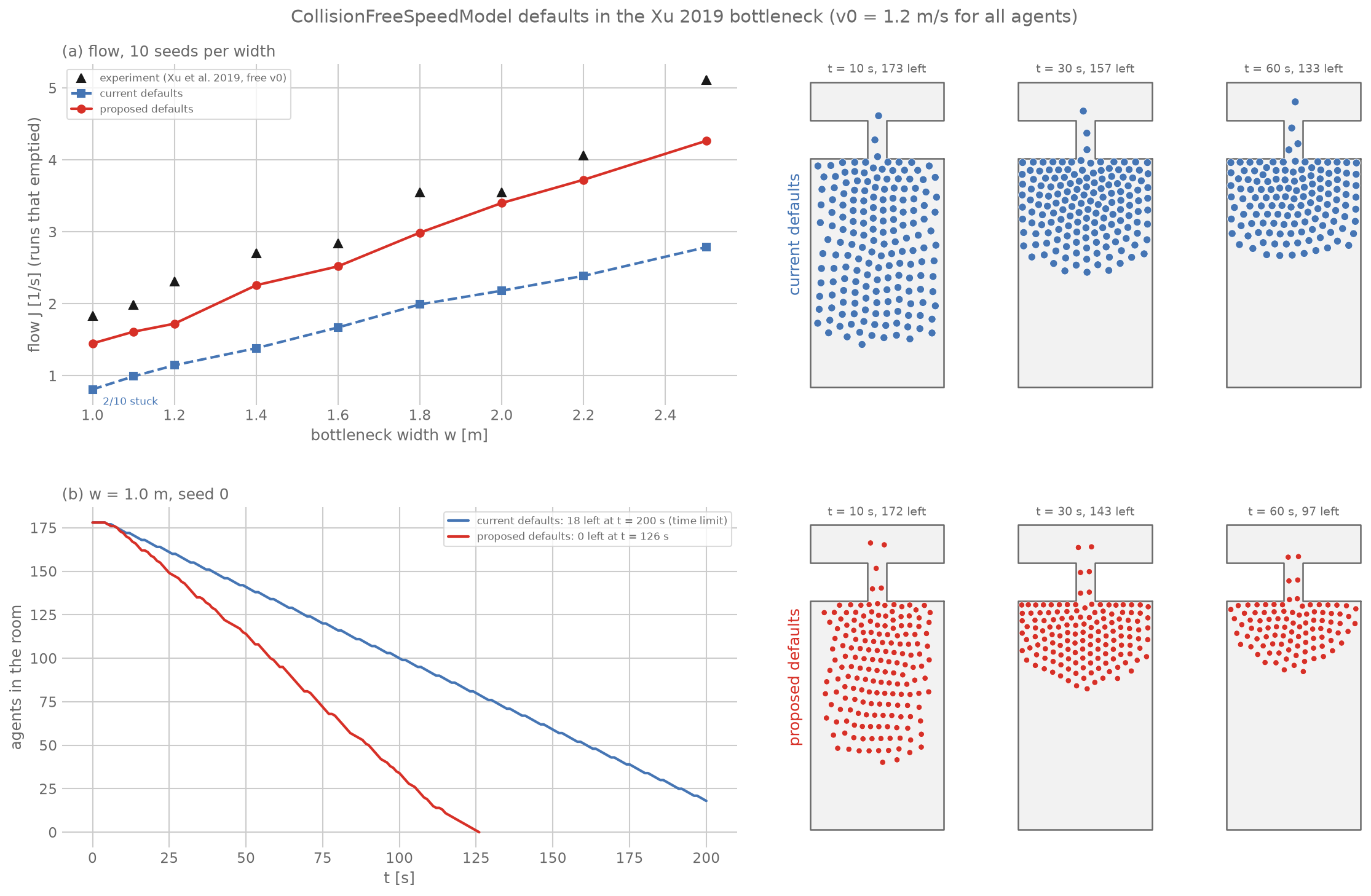
Fig. 2. The current and the proposed defaults in the bottleneck of Xu et al. (2019), all agents with a desired speed of 1.2 m/s. (a) Flow of the runs that emptied the room, 10 seeds per width. (b) Agents in the room over time at w = 1.0 m for one seed; the run with the current defaults was stopped at 200 s. Right: snapshots of the same two runs.
With the current defaults, the flow is 39 to 56 % below the experiment, and in 2 of 10 runs at 1.0 m nobody passes for 60 s. With the proposed defaults, this happens in no run, and the flow is 4 to 26 % below the experiment. In Fig. 2 (b), the proposed defaults empty the room after 126 s. The current defaults have 18 agents left after 200 s, i.e. this run is slow, not stuck.
However, the comparison is not fair to the experiment, since the participants did not all walk at 1.2 m/s. The flow is higher than with set C and the desired speeds of Xu et al. (2019) in Fig. 1 (a), probably since the slowest agents of that distribution limit the flow through the gap.
The proposed defaults change two things: the parameters of set C, and the vision factor \(\lambda = 0.5\). In order to separate them, we ran the same 1.0 m case (one seed, 1.2 m/s) with each change alone, see Fig. 3. The vision factor alone does not change the current defaults: 18 and 19 agents are left after 200 s. With the large radius and the strong repulsion of the current defaults, the agents in front of the gap stay apart and slow, and there is no jam for the vision factor to dissolve. The recalibrated parameters alone deadlock after about 34 s, and 144 agents remain until the end. The snapshot at 40 s shows the mechanism of the second section: a dense arch closes over the entrance, and the gap is empty. Only the combination empties the room, after 126 s. In other words, the recalibrated parameters make the crowd denser and faster, and the vision factor is what keeps such a crowd from blocking the gap. This agrees with the five-seed results above, where set A without the vision factor stalled in 13 of 50 runs. However, Fig. 3 shows one seed at one width.
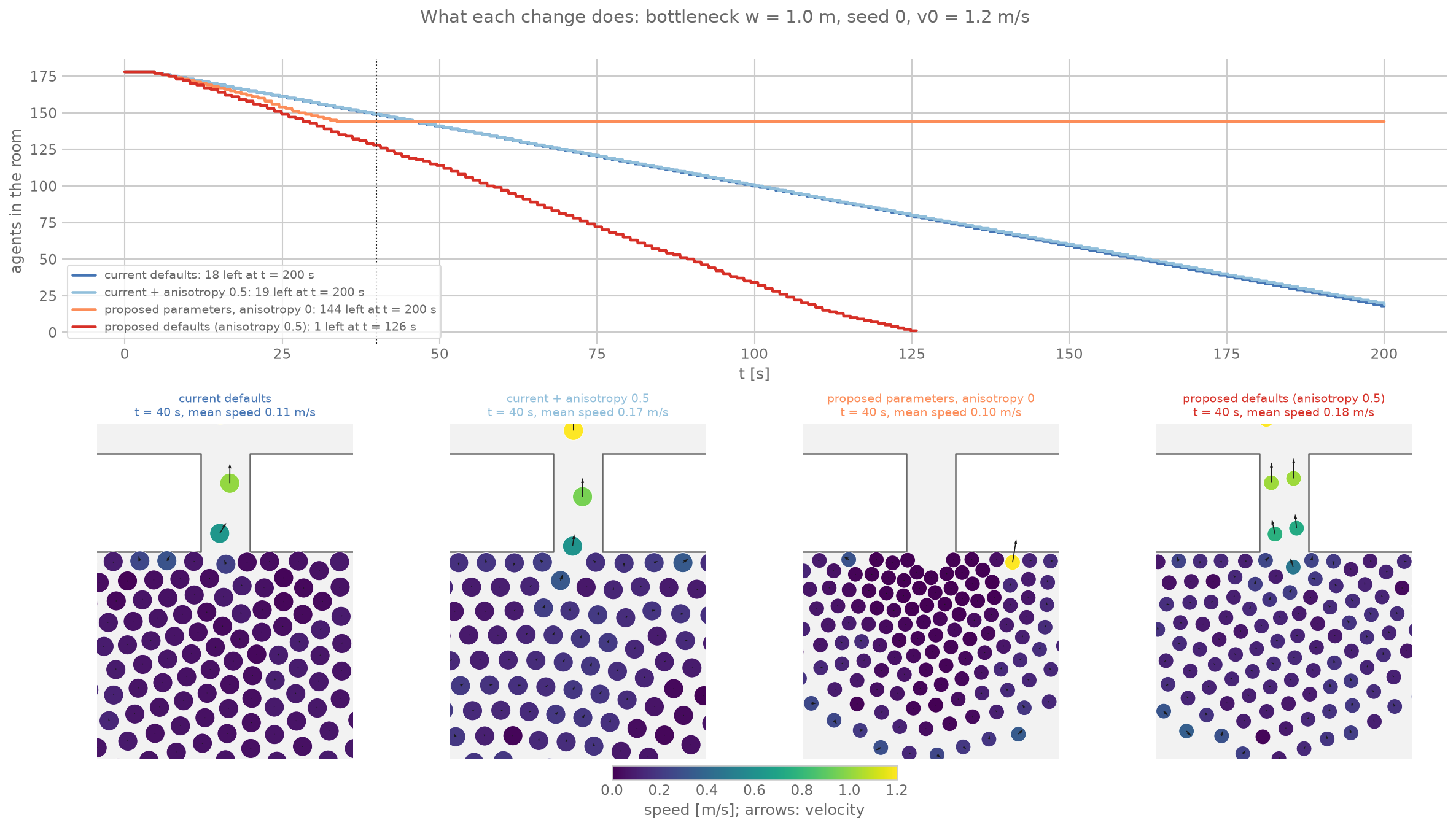
Fig. 3. The two changes separately, w = 1.0 m, one seed, all agents at 1.2 m/s. Top: agents in the room over time; the dotted line marks the snapshots. Bottom: the region around the gap at t = 40 s, colored by speed, with velocity arrows. The proposed curve ends at the last written frame, just before the last agent leaves.
A note on the time step
A fundamental diagram needs a periodic corridor, which JuPedSim does not have. We used a ring instead and a time step of 0.05 s in order to save time. A single agent in a 0.6 m wide ring then walks at 0.89 m/s instead of its desired 1.34 m/s, since the walls on both sides turn its direction back and forth. With 0.01 s, it walks at 1.34 m/s. The first fundamental diagrams were therefore wrong, including negative speeds at high density, and we discarded them. A time step that is fine in a straight corridor is not necessarily fine in a curved one. Check a single free agent before simulating a crowd.
Lessons
- Penalise the failure you care about. Without the stall term, the optimizer had no reason to prefer a set that does not clog. With it, the stall count became the main criterion between sets with similar fits.
- Re-evaluate the winner with more seeds. Two seeds selected a set that stalls in a quarter of its runs. An optimizer that sees stochastic results prefers the lucky draws.
- Test a remedy for the failure where the failure happens. The vision factor removes the deadlocks in the narrow bottleneck. In the wide Hermes bottleneck there is nothing to remove, and the full vision factor only costs accuracy. A half-weighted factor was the compromise in our data.
- A default is a compromise. No set we found meets the tolerances at both experiments. The proposed set is the most reliable one we found, not an accurate one.
Limitations
First, the calibration fixed the desired speed at 1.55 m/s, the free speed measured on the Hermes participants. The default stays at 1.2 m/s, the literature value for normal walking. Fig. 2 shows that the proposed set works at 1.2 m/s in one geometry. A calibration at 1.2 m/s would let the time gap and the repulsion absorb the faster walking of the Hermes participants, and we did not run it. Second, \(\lambda\) was not optimized; we compared the values 0, 0.5 and 1. Third, the fundamental diagrams with the 0.01 s time step have not been computed yet. Fourth, the engine errors removed about 5 % of all runs from the comparison. Despite these limitations, the proposed set is the first default of this model that is documented by a calibration and by tests on data not used for it. The defaults should be revisited when the engine errors are fixed and the fundamental diagrams are available.
References
- Chraibi, M., Seyfried, A., Schadschneider, A. (2010). Generalized centrifugal-force model for pedestrian dynamics. Physical Review E 82, 046111. doi:10.1103/PhysRevE.82.046111.
- Tordeux, A., Chraibi, M., Seyfried, A. (2016). Collision-free speed model for pedestrian dynamics. In: Traffic and Granular Flow ‘15, Springer, 225–232. doi:10.1007/978-3-319-33482-0_29.
- Xu, Q., Chraibi, M., Tordeux, A., Zhang, J. (2019). Generalized collision-free velocity model for pedestrian dynamics. Physica A 535, 122521. doi:10.1016/j.physa.2019.122521.
- Experiment data and the references of part 1 and part 2 as listed there.
Code
Driver scripts, Dakota input files and results: github.com/PedestrianDynamics/jupedsim-dakota-calibration, branch jupedsim-2.0, commit 1d7fc4e, folder joint2.
Software used in this part:
- Dakota 6.24
- JuPedSim main branch, development version of 2.0, commit 11258f0f0 (parts 1 and 2: release 1.4.2)
- PedPy 1.5.1
By: Mohcine Chraibi