How do you validate a pedestrian model against real data?

How do you validate a pedestrian model against real data?

We calibrated JuPedSim’s Collision Free Speed model with Dakota against one open bottleneck experiment and tested the result on two others, all with the same open analysis code. The defaults miss the measured flow by a factor of two. Calibration fixes that at the wide bottleneck, mostly within ten percent on flow, density and speed, including at two widths the optimizer never saw. The same parameters then fail at a half-metre gate and at an unguided entrance, two optimizer runs give two different “best” sets, and low motivation is not something a static parameter reproduces. Along the way we found five mistakes in our own pipeline and a speed observable that was partly measuring tracking noise. The note walks through the procedure step by step so that it can be repeated, and closes with what we would do differently. If you only read one section, read the lessons at the end.

Pedestrian simulations are used to size exits, plan events and argue about safety, so the question whether a model is right is not academic. The simulation community settled the vocabulary long ago. Verification asks whether the software implements the model correctly. Validation asks whether the model, within the domain it is meant for, reproduces reality with an accuracy that is good enough for its purpose (Sargent 1984, 2008; ISO 16730 as summarised by Ronchi et al. 2013). Sargent adds two points that are easy to forget: a model is never valid in the abstract but only for a purpose, and confidence in a model costs money, so one always stops somewhere short of certainty.

In pedestrian dynamics the models multiplied faster than the data to test them. Seyfried and Schadschneider (2008) showed that even the fundamental diagram, the most basic relation of the field, differs between handbooks by a factor of two in capacity, and that part of the discrepancy comes from the measurement method rather than the crowd. Reliable validation data were so scarce that Oh et al. (2014) validated a bottleneck model with mice. The NIST review of evacuation model verification and validation (Ronchi et al. 2013) lists the open questions bluntly: what accuracy counts as good enough, how many tests, and who runs them.

Two lessons from this field’s own validation work shape what follows. Liao et al. (2014) calibrated FDS+Evac on the very experiment we use here, by hand, to match the flow at one width. The flow matched. The density in front of the bottleneck was too low and the speed too high, so the model reached the right flow for the wrong reasons. Their follow-up (Liao et al. 2017) turned that into a rule: a single characteristic cannot validate a model, and the comparison has to combine several. Kurtc et al. (2018) drew the second lesson: the assessment should be automated, including the search for parameters, or it will not be done consistently.

A recent study by Kretz et al. (2026) reached the first lesson from the other side. They calibrated the social force model in PTV Viswalk on their own bottleneck experiment, 45 participants cycling through a room with a 0.6 m exit, by fitting a single parameter to the mean flow with a grid search over a thousand seeds per candidate. The flow matched either way. What separated a good calibration from a bad one only showed up in the individual travel times recorded with RFID tags: with one common relaxation time for all agents, the slow ones waited at the exit until everyone else had passed, one agent was overtaken by 116 others where the experiment showed at most 15. Fixing the base acceleration instead and deriving the relaxation time per agent removed most of that without touching the flow. Two things carry over to what follows. Their argument that desired speed and relaxation time are only identified through their ratio is the same degeneracy we meet below between desired speed and time gap. And their evaluation observable, the distribution of travel times and of rank changes between entry and exit, is one we do not use; it is computable from our trajectories and would test the upstream state from the microscopic side. Their study has no held-out runs and one geometry, which they state; ours holds widths out and changes the experiment, but measures only the aggregate state in front of the opening.

This note puts the two together with tools that are open and generic. The simulation is JuPedSim, the analysis of experiment and simulation alike is PedPy, and the screening, sensitivity analysis and calibration are run by Dakota, Sandia’s toolkit for exactly this kind of study. Dakota has been used in engineering for decades and almost never in pedestrian dynamics. It turns “which parameters matter, and what values fit the data” from a pile of private scripts into a text file.

What validation means here

Following Sargent, we state the purpose first. The model should reproduce the flow through wide bottlenecks in a dense, motivated crowd, and it should do so with the right density and speed in front of the bottleneck, not only the right flow. Three observables therefore enter every comparison: they are the complementary quantities we chose for this study, throughput and the two components of the upstream state, not a canonical minimum. The decision rule is a fixed relative tolerance per observable, 6 % on flow and 10 % on density and speed, and a comparison passes when the mean over simulation seeds lies within it. The same numbers were used as the uncertainties that weight the calibration residuals; they were set before any calibration was run, from the seed-to-seed spread of the simulation plus an allowance for measurement error, but they were chosen as calibration weights, and adopting them as the acceptance tolerance is a decision we made when the results were assessed, not a pre-registered one. The validation data are held out: the optimizer sees three bottleneck widths and never the other two.

Step 1 — the experiment

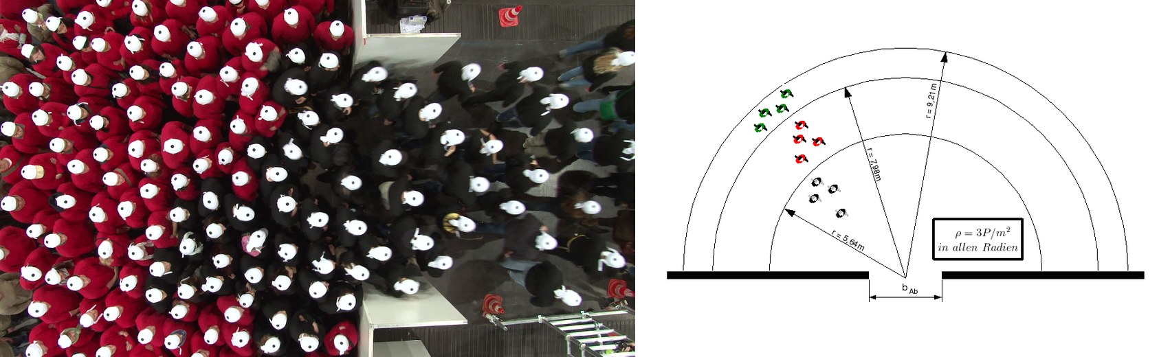
The Hermes bottleneck experiment, Düsseldorf 2009: overhead view of a run, and the setup sketch with the semicircular holding zones at 3 persons per square metre. Images: Pedestrian Dynamics Data Archive, Forschungszentrum Jülich.

The Hermes bottleneck experiment, Düsseldorf 2009: overhead view of a run, and the setup sketch with the semicircular holding zones at 3 persons per square metre. Images: Pedestrian Dynamics Data Archive, Forschungszentrum Jülich.

The Hermes bottleneck experiment was run in May 2009 in Hall 2 of the Düsseldorf fairground with about 350 participants (Seyfried et al. 2009; Liao et al. 2014). The bottleneck was built from boards higher than two metres, 1 m long, and its width was varied from 2.4 to 5.0 m in five runs. Participants waited in a semicircular holding area of radius 8.6 m directly in front of the bottleneck, which puts the initial density at three persons per square metre, and walked through on command. The free walking speed of 42 participants was measured separately: 1.55 m/s with a spread of 0.18 m/s.

The trajectories are open data with a DOI. Since 2024 they come as HDF5 files that carry a geometry along, so PedPy loads both with one call each. One caveat, found only by reading the paper next to the file: the polygon in the archive is a 12 m box around the camera window with the wall blocks cut off at its edges, and three of its five gaps are 0.1 m narrower than the run’s stated width. The simulation therefore takes the gap width from the run parameter and the corridor and holding area from the paper. A corrected polygon for each run is in the repository.

import pedpy, pathlib
f = pathlib.Path("ao-360-400.h5")
traj = pedpy.load_trajectory_from_ped_data_archive_hdf5(f)
area = pedpy.load_walkable_area_from_ped_data_archive_hdf5(f)

We measure three things per run: the flow through the bottleneck, from the slope of the N(t) curve at a line across the gap; and the density and mean speed in a 2.8 by 2 m area directly in front of it, averaged over the jam phase. The area is the same for all widths, so it covers more than the 2.4 m opening and only the middle of the 5.0 m one. These are local measurements of the crowd state upstream of the gap, not averages over the whole opening, and the calibration compares them like for like. The same three functions are applied to the simulated trajectories. Seyfried and Schadschneider’s warning about measurement methods is answered the simplest way: there is only one method, applied to both sides.
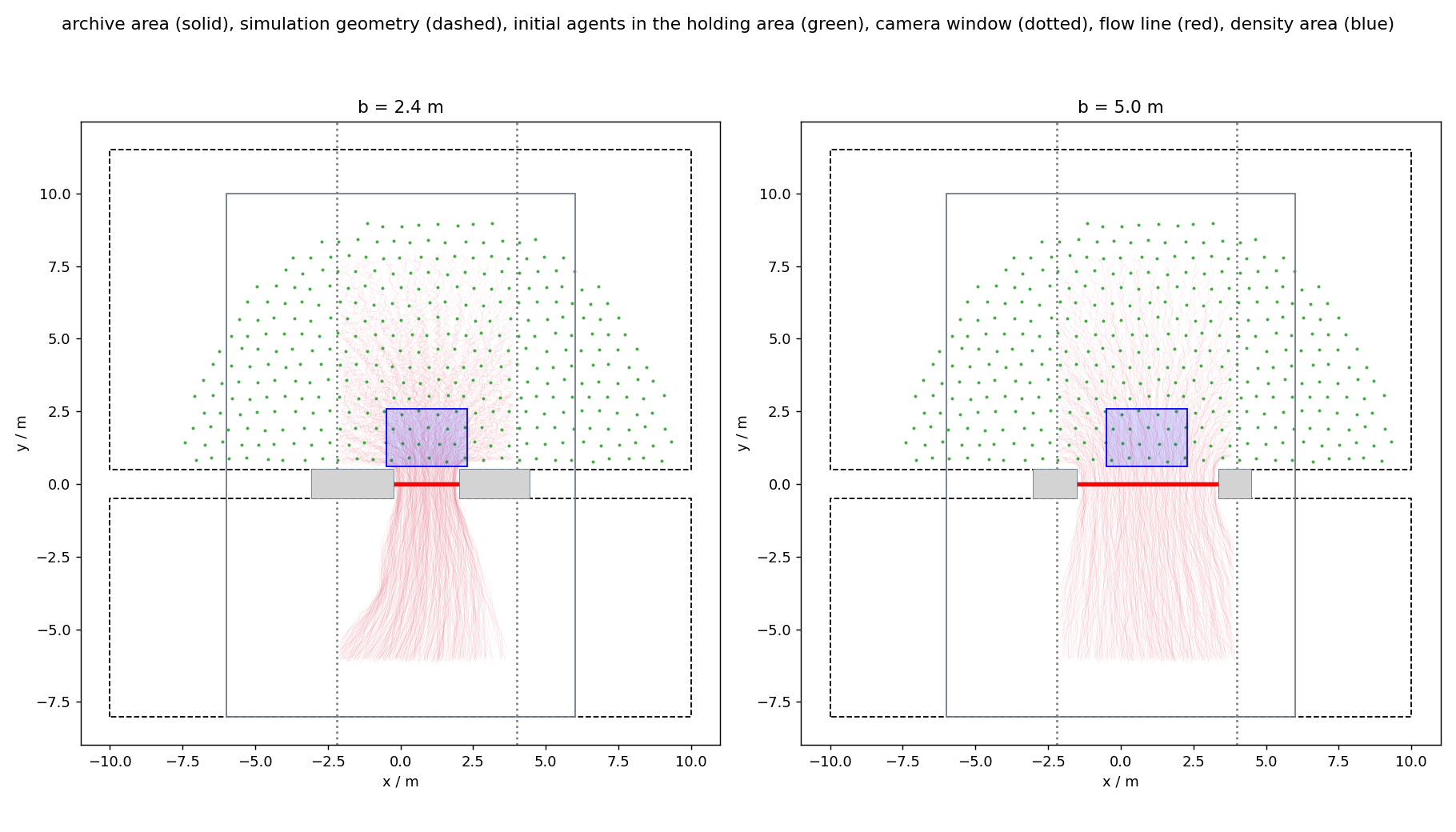
Measurement setup for the 2.4 m and 5.0 m runs. Red: the flow line across the gap. Blue: the area for density and speed. The dashed line is the simulation geometry: a 20 m wide corridor with the bottleneck boards as a wall band. The dotted lines mark the camera window of the experiment.

Measurement setup for the 2.4 m and 5.0 m runs. Red: the flow line across the gap. Blue: the area for density and speed. The dashed line is the simulation geometry: a 20 m wide corridor with the bottleneck boards as a wall band. The dotted lines mark the camera window of the experiment.

Step 2 — the defaults are wrong by a factor of two

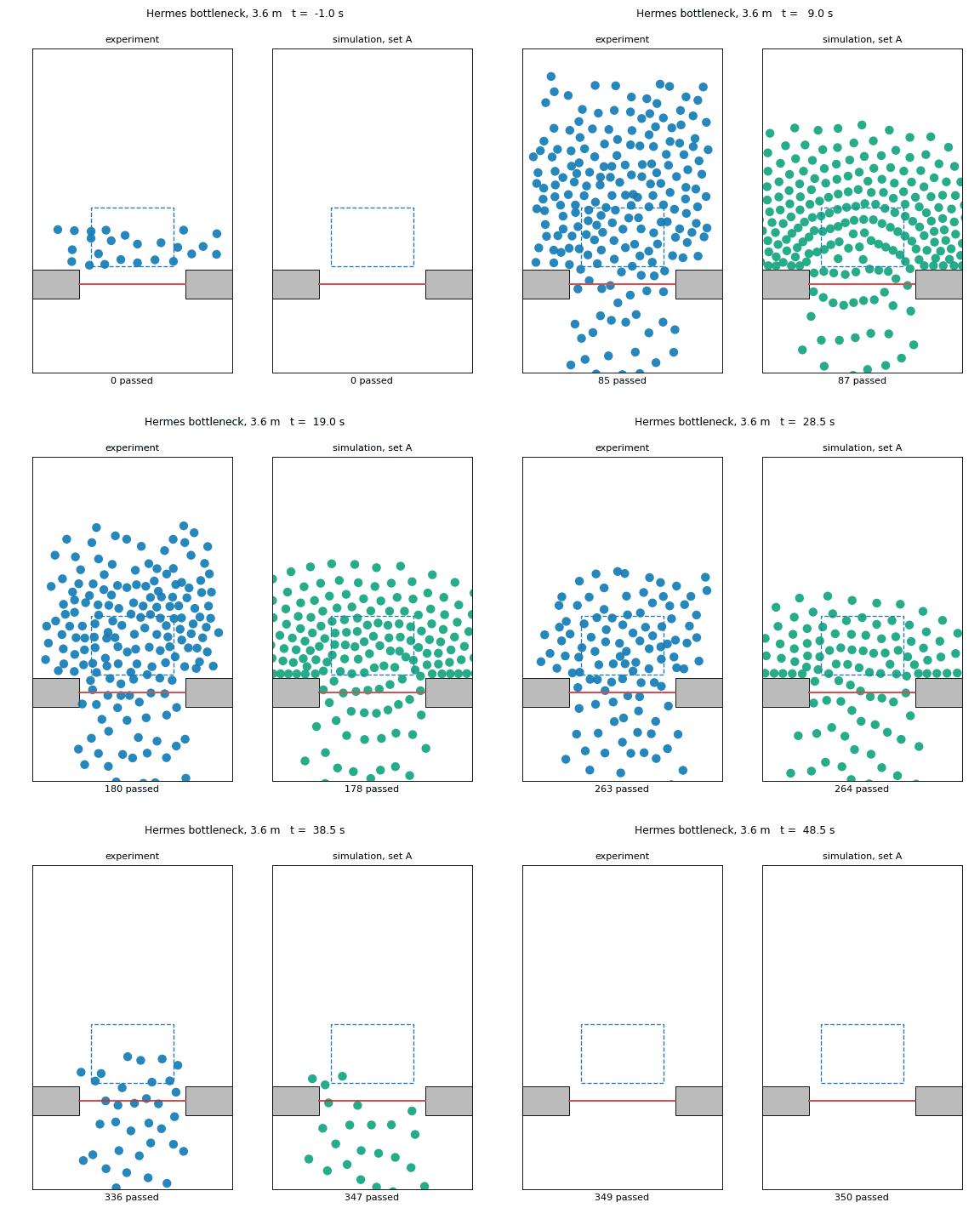
We rebuilt the setup in JuPedSim: the corridor, the boards, the semicircular holding area with 350 agents at three per square metre, and an exit line behind the bottleneck. The model is the Collision Free Speed model (Tordeux et al. 2016) with its default parameters.
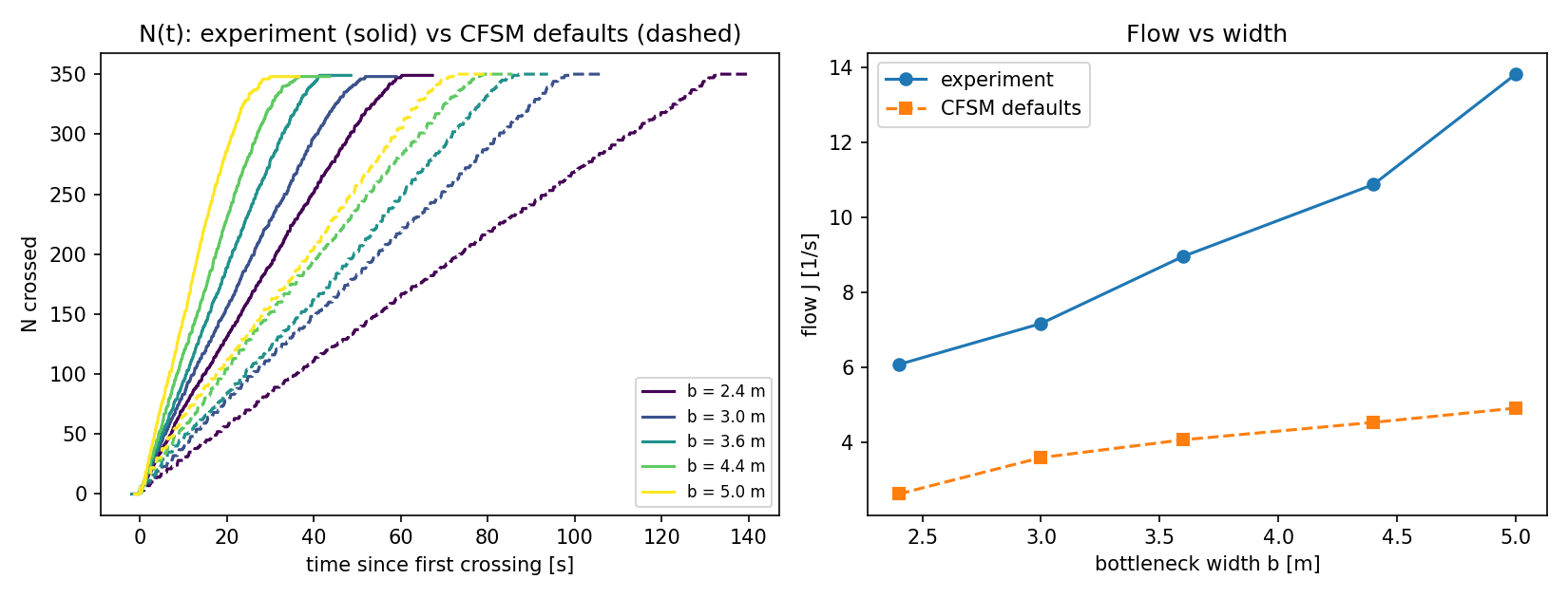
Measured N(t) curves (solid) against the default model (dashed), and flow against bottleneck width. The defaults underpredict the flow by a factor of two to three, worst at the widest opening.

Measured N(t) curves (solid) against the default model (dashed), and flow against bottleneck width. The defaults underpredict the flow by a factor of two to three, worst at the widest opening.

This is not a surprise if you know the model. In the Collision Free Speed model the time gap sets the headway an agent keeps to the one in front, and the radius sets how close agents can pack side by side; together with the neighbor repulsion they fix the throughput of a jammed opening, and the desired speed hardly enters once the crowd is jammed. With the defaults, one second of headway and a 0.2 m radius, the model delivers a third to a half of the measured flow. No amount of tweaking the desired speed fixes that. The question is which of the seven parameters do, and by how much.

Step 3 — let Dakota find the parameters that matter

Dakota needs two things: an input file describing the study, and a driver script that turns a parameter vector into responses. Our driver reads Dakota’s parameter file, runs one JuPedSim simulation per bottleneck width, computes the three observables with PedPy and writes them back. That is all the coupling there is.

method
  psuade_moat
    samples = 160
    partitions = 3

variables
  continuous_design = 7
    descriptors 'desired_speed' 'radius' 'time_gap' 'strength_neighbor'
                'range_neighbor' 'strength_geometry' 'range_geometry'
    lower_bounds 0.8 0.12 0.10  2.0 0.02  1.0 0.01
    upper_bounds 1.8 0.25 1.20 15.0 0.50 10.0 0.20

interface
  fork
    analysis_drivers = 'python3 driver.py'
    parameters_file = 'params.in'
    results_file = 'results.out'
    work_directory named 'runs/run' directory_tag
  asynchronous evaluation_concurrency = 3

responses
  response_functions = 9
  no_gradients
  no_hessians

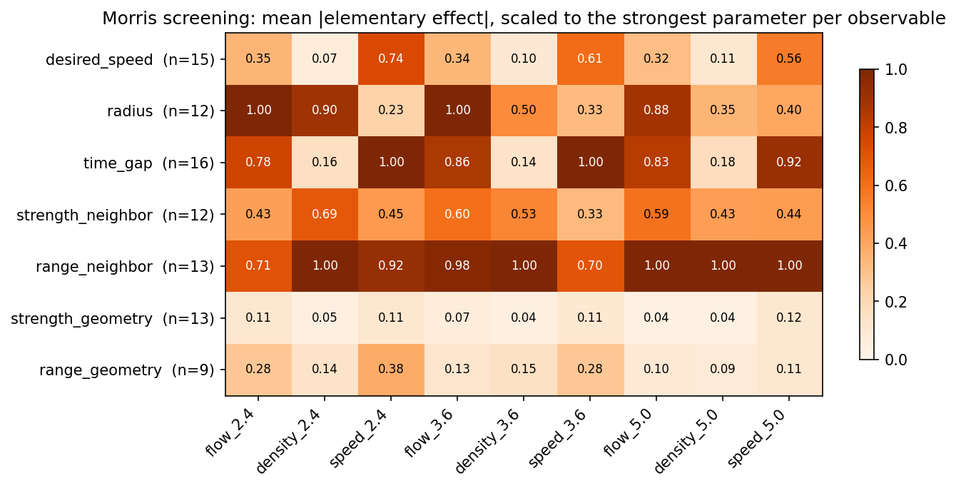
The first stage is a Morris screening: twenty trajectories of eight evaluations each, every step changing one parameter at a time, 160 evaluations in all. It is cheap and it ranks the parameters per observable. It is a ranking, not a measurement, and any ranking of this kind is conditional on the ranges it was sampled over. We ran it first with ten trajectories and then with twenty; the broad pattern was the same, with some reordering among the mid-ranked parameters, so the figure shows the larger run.
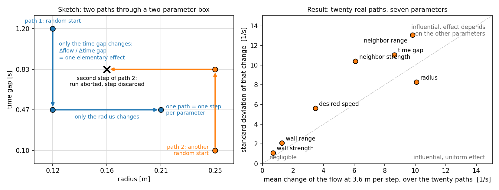
Morris screening over the full parameter ranges, twenty trajectories. Each cell is the mean absolute elementary effect of a parameter on an observable, scaled to the strongest parameter in that column. An elementary effect is one step of one parameter along a trajectory; steps where either end failed were discarded, and n per row is the number of valid steps that survived out of the twenty drawn. The time gap, the radius and the neighbor repulsion range dominate; the desired speed has a moderate effect on flow and speed over this wide range; the two wall parameters are weakest.

Morris screening over the full parameter ranges, twenty trajectories. Each cell is the mean absolute elementary effect of a parameter on an observable, scaled to the strongest parameter in that column. An elementary effect is one step of one parameter along a trajectory; steps where either end failed were discarded, and n per row is the number of valid steps that survived out of the twenty drawn. The time gap, the radius and the neighbor repulsion range dominate; the desired speed has a moderate effect on flow and speed over this wide range; the two wall parameters are weakest.

The screening also revealed something no fit would have: in 43 of the 160 evaluations, about a quarter, the model pushed agents through the walls and JuPedSim aborted the run. Those combinations have strong, long-range neighbor repulsion and weak wall repulsion. We narrowed the bounds accordingly and froze the wall parameters at their defaults. Knowing where a model breaks is part of validating it.

With five parameters left, and narrower ranges, a Sobol analysis gives the variance decomposition. Dakota computes the indices itself; the input file changes from the Morris method block to a sampling block with the keyword variance_based_decomp, the variables become uncertain variables with uniform distributions over the narrowed ranges, and the cost is the base sample size times the number of parameters plus two. Each parameter point uses simulation seed 1; seed variability is measured separately later rather than being treated as another physical input. Because the ranges and the fixed parameters changed between the two stages, the two rankings are not expected to coincide exactly; sensitivity is always relative to the ranges assumed.

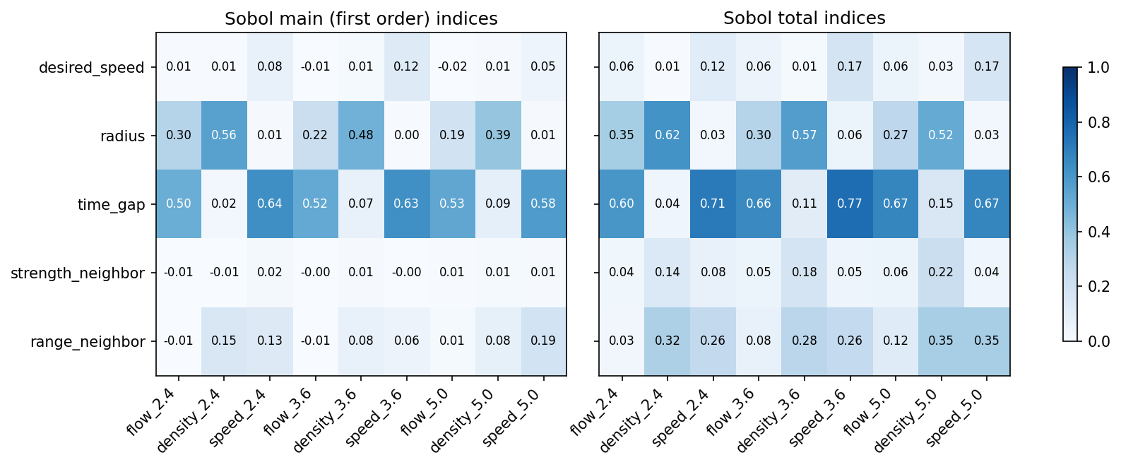
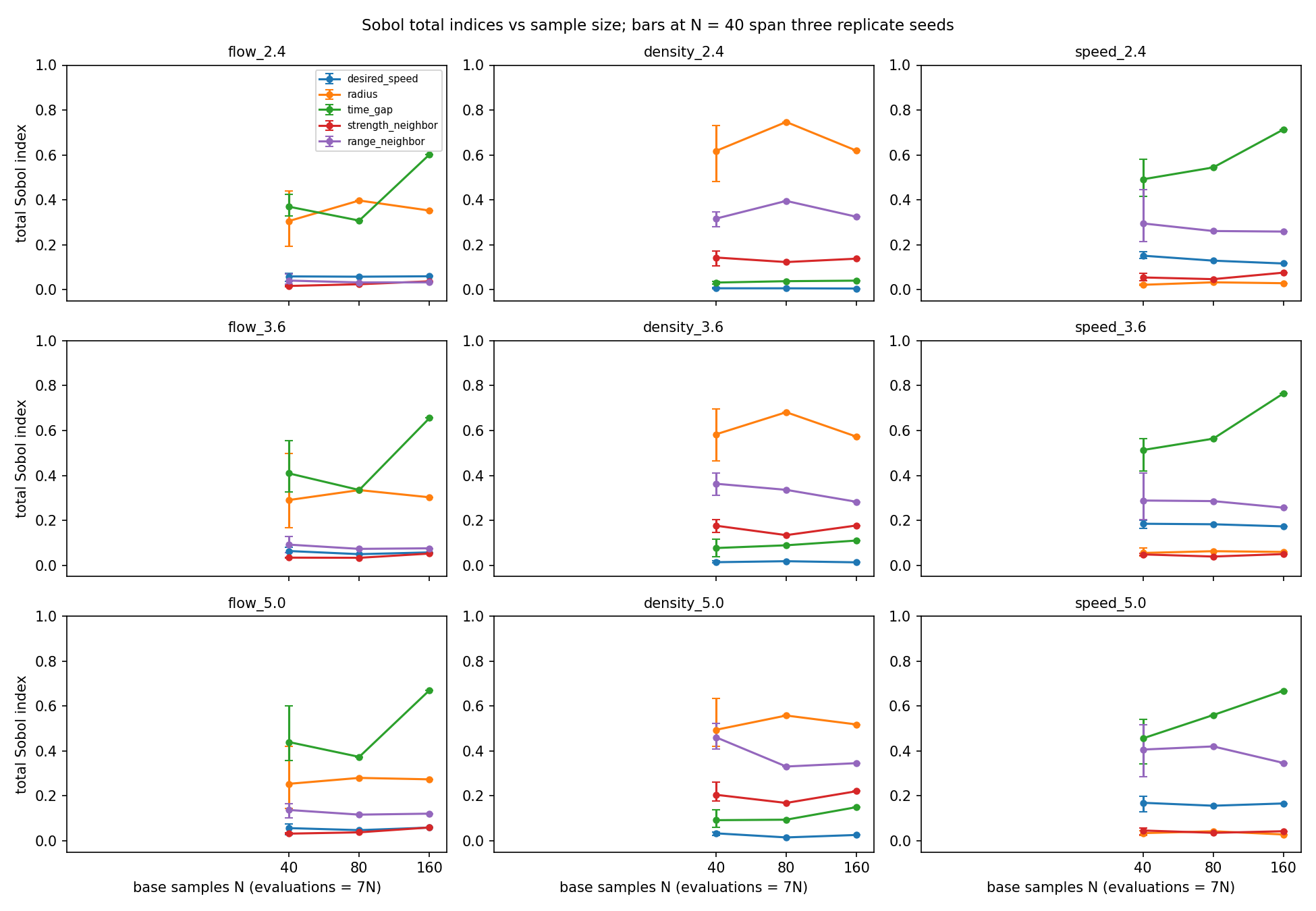
How many samples are enough is an empirical question, so we answered it empirically: three replicate runs with 40 base samples and different seeds, then 80 and 160 base samples, 2520 evaluations in all. In the original 40-base-sample run, 18 of the 45 first-order indices exceeded their totals; the two replicate runs had 11 and 13 such violations, which exact indices cannot do. At 160 samples, two estimates still exceeded their totals, but only by 0.0016 and 0.000014, so there were no material violations. But the estimates are not converged: the time gap’s total index on flow and speed still rises from about 0.4 to about 0.7 between 80 and 160 samples, and at 2.4 m the radius leads the time gap for flow at 80 samples while the time gap leads at 160. What is stable across every run is the small group of influential parameters per observable: time gap and radius for flow, radius and neighbor range for density, time gap and neighbor range for speed, with the desired speed a minor contributor and the neighbor strength minor except for density. The ordering within those groups and the magnitudes are provisional, and since only the grouping is used below, we did not spend further computation on them.

Sobol indices for the five remaining parameters from the run with 160 base samples, 1120 evaluations, none failed. The time gap dominates flow and speed with total indices of 0.6 to 0.8; the radius dominates density with 0.5 to 0.6, followed by the neighbor repulsion range with about 0.3; the neighbor range also contributes 0.25 to 0.35 to speed; the desired speed contributes 0.06 to flow and 0.12 to 0.17 to speed. Two first-order estimates exceed their totals by 0.0016 and 0.000014; these are numerical estimation noise, not material violations.
Sobol indices for the five remaining parameters from the run with 160 base samples, 1120 evaluations, none failed. The time gap dominates flow and speed with total indices of 0.6 to 0.8; the radius dominates density with 0.5 to 0.6, followed by the neighbor repulsion range with about 0.3; the neighbor range also contributes 0.25 to 0.35 to speed; the desired speed contributes 0.06 to flow and 0.12 to 0.17 to speed. Two first-order estimates exceed their totals by 0.0016 and 0.000014; these are numerical estimation noise, not material violations.

Sobol total indices against the base sample size. Bars at 40 span three replicate runs with different seeds. The group of influential parameters per observable is the same in every run; the magnitude of the time gap’s index and its order relative to the radius for flow are not settled at 160 base samples, so the values are provisional.

Sobol total indices against the base sample size. Bars at 40 span three replicate runs with different seeds. The group of influential parameters per observable is the same in every run; the magnitude of the time gap’s index and its order relative to the radius for flow are not settled at 160 base samples, so the values are provisional.

Step 4 — calibration, and why we did not use gradients

Our first attempt at calibration, on a simpler two-room test case before touching the experiment, used Dakota’s gradient-based least-squares solver with finite-difference gradients. It stalled at the starting point: two simulations whose parameters differ in the sixth digit produced evacuation times that differed by seconds, and the differences used as gradients were noise. We did not repeat the experiment on the Hermes objective, so this is an observation about that solver configuration on that test, not a demonstrated property of the calibration problem here.

The method we used instead is Dakota’s efficient_global: it fits a Gaussian process to the evaluations so far and picks the next point where the expected improvement is largest. It needs no gradients, it copes with noise, and it treats each evaluation as expensive, which ours are. We calibrated on the 2.4, 3.6 and 5.0 m runs, nine residuals weighted by their uncertainty, and kept the 3.0 and 4.4 m runs untouched for validation.

method
  efficient_global
    max_iterations = 60

responses
  calibration_terms = 9
    weights = 7.6 3.2 977  3.4 4.3 517  1.45 6.0 252
  no_gradients
  no_hessians

After 42 evaluations, about twenty minutes on a laptop, the optimizer converged with all nine residuals below one standard deviation of the assumed uncertainty. And the desired speed had gone to the lower bound of its range, 0.8 m/s, half the free speed measured on the participants.

This is the moment where a fit and a validation part ways. The Sobol analysis had already said that the desired speed is a minor influence on the jam observables, so the misfit is flat along it and the optimizer was free to put it wherever the residuals were a hair smaller. A model with participants walking at 0.8 m/s reproduces the bottleneck. It does not reproduce the participants. Sargent calls this data validity: parameters that were measured are data, not fitting variables. Liao et al. (2014) made the same move for FDS+Evac. So we fixed the desired speed at the measured 1.55 m/s and calibrated the remaining four parameters. That converged in 24 evaluations.

parameterdefaultall five freespeed fixed, set Aspeed fixed, set B
desired speed [m/s]1.20.80 (at bound)1.55 (measured)1.55 (measured)
radius [m]0.200.140.130.15
time gap [s]1.00.560.810.55
neighbor repulsion strength86.12.19.4
neighbor repulsion range [m]0.100.150.250.10
weighted residual norm (six-seed recalculation)2.72.4

Set B is the reason for the last column. Because a surrogate-based optimizer with a few dozen evaluations can settle in one region of a flat landscape, we repeated the fixed-speed calibration from a different optimizer seed as a robustness check. Dakota reported objective norms of 1.0 and 1.5 at the selected evaluations. Recomputing the norm from the six-seed means used for the later comparison gives 2.7 for set A and 2.4 for set B; those are the values in the table. The difference is below what the seed-to-seed noise of the simulation can resolve. The first run had visited the same region on its way and rated it 2.9. So there are at least two calibrated parameter sets for this experiment that the data cannot choose between. Two starts say nothing about the shape of the objective in between; they show that the reported optimum depends on where the optimizer started.

All these sets reproduce flow and density at the three calibration widths to within about ten percent, and speed to within twenty. They are nowhere near each other. Time gap, repulsion strength and range shift by factors of two to four between them. Three observables at three widths do not pin five parameters, and a good fit says nothing about whether the parameters mean what their names say. Fixing the one parameter that was measured removes the freedom to be wrong in that direction. It does not make the others physical: the radius that comes out, 0.13 to 0.15 m, is an effective size in a model with round bodies, and the remaining parameters still compensate for one another.

Step 5 — does it hold on the widths it never saw?
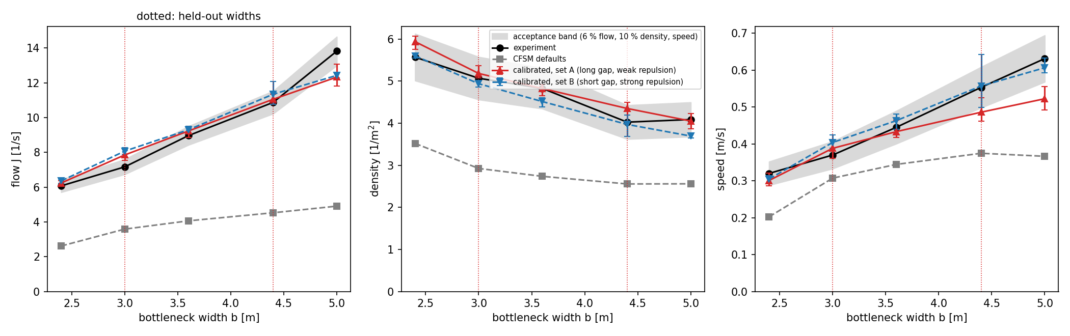
Flow, density and speed against bottleneck width: experiment with the acceptance band (6 % on flow, 10 % on density and speed, the uncertainty assumed in the calibration weights), default model, and the two calibrated sets with the desired speed fixed. Error bars are the minimum and maximum over six simulation seeds; the experiment is one run per width. The dotted widths, 3.0 and 4.4 m, were not used in the calibration.

Flow, density and speed against bottleneck width: experiment with the acceptance band (6 % on flow, 10 % on density and speed, the uncertainty assumed in the calibration weights), default model, and the two calibrated sets with the desired speed fixed. Error bars are the minimum and maximum over six simulation seeds; the experiment is one run per width. The dotted widths, 3.0 and 4.4 m, were not used in the calibration.

With the desired speed fixed, both calibrated sets improve every observable substantially, at the held-out widths too, and the figure shows the acceptance tolerance, 6 % on flow and 10 % on density and speed. Applied as a decision rule, neither set passes everywhere. Both overshoot the flow at the held-out 3.0 m by 10 to 13 %; set A’s speed is 12 % low at the held-out 4.4 m; and at the 5.0 m calibration width both are 10 % low on flow. Where the two sets differ is what else they get wrong at the wide end. Set A follows the measured increase of speed with width up to 3.6 m and then flattens, 17 % low at 5.0 m, while it keeps the density within tolerance. Set B keeps the speed within tolerance at every width and instead lets the density fall 10 % short at 5.0 m. So at the widest opening set A preserves the local density and underpredicts the speed, set B improves the speed and underpredicts the density, and both underpredict the flow. That is a milder version of what Liao et al. (2014) saw in FDS+Evac.

Deviation of the simulation from the experiment, mean over six seeds, with the band at 6 % for flow and 10 % for density and speed:

width [m]flow A / Bdensity A / Bspeed A / B
2.4+3 % / +5 %+7 % / +1 %−6 % / −5 %
3.0 (held out)+10 % / +13 %+2 % / −3 %+5 % / +9 %
3.6+3 % / +4 %0 % / −6 %−3 % / +4 %
4.4 (held out)+2 % / +4 %+8 % / −1 %−12 % / +1 %
5.0−11 % / −10 %−1 % / −10 %−17 % / −4 %

The seed-to-seed standard deviation is 2 to 4 % for flow and density and 3 to 6 % for speed, so the differences between A and B at the wide openings are larger than the simulation noise.

So the honest summary of Step 5 is: a substantial improvement over the defaults, but the model is not validated for the full 2.4 to 5.0 m range by the stated rule. At the calibration widths 2.4 and 3.6 m both sets meet the tolerance on all three observables, which is a fit, not validation. The held-out evidence is two widths: at 4.4 m set B meets the tolerance on all three observables and set A fails it on speed; at 3.0 m both fail it on flow. And both miss the widest calibration opening in a way the two calibrations move between speed and density but neither removes. Whether that is acceptable depends on the purpose, which is exactly why the purpose has to be stated first.

Step 6 — a second experiment, and where the model stops

The CrowdQueue experiment, Wuppertal 2018: a run in the 5.6 m corridor seen from above, and the setup with the 0.5 m gate at the origin. Images: Pedestrian Dynamics Data Archive, Forschungszentrum Jülich.

The CrowdQueue experiment, Wuppertal 2018: a run in the 5.6 m corridor seen from above, and the setup with the 0.5 m gate at the origin. Images: Pedestrian Dynamics Data Archive, Forschungszentrum Jülich.

A calibration is only validated within the domain it was tested in. To find the edge of that domain we took a second open dataset, the CrowdQueue experiment from Wuppertal 2018 (Adrian et al. 2020): a crowd in front of an entrance again, but through a 0.5 m gate instead of a 2.4 to 5 m opening, in corridors from 1.2 to 5.6 m wide, with 11 to 75 participants and the motivation varied between runs. The archive files carry the full geometry and every trajectory, and each simulation is seeded from the data: agents that are in view at the first frame start there, and agents that enter the tracked corridor later are injected at the time and place of their first observation. Every tracked participant is simulated; the archive’s participant counts and the tracked counts agree for all 21 usable runs. An injection that finds its spot occupied is retried with small displacements for 10 s and then dropped; this happened to one to four people in a few seeds of the two densest 1.2 m runs, and such a seed cannot count as emptied because the expected population, the tracked count, was not all simulated. The simulated area is the corridor and the space behind the gate only. Density and speed use the same window in experiment and simulation, the frames between the tenth and ninetieth percent of that run’s own crossings, so a simulation that discharges more slowly is averaged over a longer window than the experiment. Density is the time average over every frame; speed is averaged only over frames in which the area is occupied. An earlier version averaged the zeros that PedPy returns for empty frames and consequently reported 0.12 m/s rather than 0.56 m/s for the sparse high-motivation run, whose area is empty in 78 % of its measurement frames. Whether an observable is conditional on occupancy is part of its definition, and sparse runs expose the difference. The flow is measured at a gate line, whereas density and speed are averaged in a 2.2 m² upstream area and are not a same-cross-section flux identity; the three values should therefore not be forced to satisfy (q=\rho v).

A note on what checking this section cost. A review of an earlier draft asked whether the simulations really contained everyone in the experiment, and they did not. Two of the runs have a third of their participants entering the tracked corridor during the first seconds, after the first frame from which we had taken the starting positions; one of those runs was in the calibration set. The same audit found that the trajectory writer buffers its last hundred frames and writes them only when it is closed, which we had not done, so the last few seconds of every simulation in this note had been missing from the analysis, and it found that a full-width exit region let the router send agents around the outside of the barriers. All three were corrected, and every CrowdQueue calibration and comparison below, the semicircle runs, and the Hermes validations were recomputed. The Hermes calibrations and the sensitivity analyses use steady-phase observables, and we checked rather than assumed that the lost seconds do not touch them: for the default and the calibrated parameters at three widths, deleting the last hundred written frames from a complete trajectory changes the crossing count by at most two of 350, the measurement window by at most 0.3 s, and flow, density and speed by at most 0.4 %. Those analyses were kept. We report this because validation that does not audit its own pipeline is not validation.

Each run is simulated three times and every seed is shown, because averages hide the thing that matters here. A seed counts as emptied if every expected participant was injected and passed the gate within 120 s, twice the longest experiment. Otherwise it is not emptied, and if it also had an interval of 20 s or more without a crossing while agents remained, it counts as stalled. Flow is the slope of N(t) between the tenth and ninetieth percent of crossings for emptied runs; for runs that did not empty it is the number who passed divided by the time from the first crossing to the end of the run, which is lower by construction. Both are given in the repository; the figure shows the one that was calibrated on.

N(t) at the gate for three baseline runs, experiment against the three seeds of CrowdQueue set C. The simulated slopes are steeper than the measurements. In run 110 each seed passes 62 of 63 tracked participants because one late entrant could not be placed; none is classified as stalled.

N(t) at the gate for three baseline runs, experiment against the three seeds of CrowdQueue set C. The simulated slopes are steeper than the measurements. In run 110 each seed passes 62 of 63 tracked participants because one late entrant could not be placed; none is classified as stalled.

The transfer test comes first: the two Hermes parameter sets applied to the 21 runs without refitting. Set A, the long time gap with weak long-range repulsion, stalls at the funnel in 46 of 63 seeds and empties 16. Set B, the short gap with strong short-range repulsion, empties 59 of 63 and stalls in none, but where it flows it overshoots the measured gate flow by 22 % on average in the baseline runs and by 37 % in the low-motivation runs. So of the two Hermes optima that the wide-bottleneck data could not tell apart, one mostly stalls at a half-metre gate and the other passes it too fast. That is the practical meaning of the parameter compensation in Step 4: sets with the same fit quality on one experiment behave differently on another.

Recalibrating on the seven baseline runs at 1.2, 3.4 and 5.6 m, with the wall parameters free because the 1.2 m corridors exercise them, was done from two optimizer starts as in Step 4, and again they disagree. Set C has a three-seed norm of 11.3 on its calibration runs and empties 59 of 63 seeds over all conditions; four late entrants could not be placed. Set D has a norm of 16.2 on the calibration runs and, over all conditions, stalls in 14 seeds and fails once. Set C’s baseline flows are 12 % high on average, with individual runs from 2 % low to 30 % high. Its radius is 0.124 m; set D puts radius almost at its 0.10 m lower bound. A second optimizer start changed both the inferred parameters and whether the narrow gate remained passable.

CrowdQueue: experiment (bars) against Hermes set B transferred without fitting (blue), the CrowdQueue calibration, set C (orange), and the joint calibration (green), one marker per seed, columns ordered by corridor width with the run number; asterisks mark the runs used in the calibration. Filled circle: the run emptied within 120 s; open circle: not emptied, discharge continuing; open square: stalled. Top: baseline motivation, bottom: low motivation.

CrowdQueue: experiment (bars) against Hermes set B transferred without fitting (blue), the CrowdQueue calibration, set C (orange), and the joint calibration (green), one marker per seed, columns ordered by corridor width with the run number; asterisks mark the runs used in the calibration. Filled circle: the run emptied within 120 s; open circle: not emptied, discharge continuing; open square: stalled. Top: baseline motivation, bottom: low motivation.

The low-motivation runs show what a flow-only validation would miss. Between the baseline and the low-motivation condition the measured flow at the same gate is about 10 % lower; the model has no input for motivation, so with parameters fixed at the baseline calibration it predicts the same or a higher flow, and overshoots the low-motivation runs by 24 % on average. In the 1.2 m corridor with 24 people, set C gives a flow 29 % high, a front area 44 % denser than measured and people moving 21 % slower: throughput alone hides two compensating errors in the upstream state.

What static parameters can absorb

The corrected seven-parameter fits are condition-specific, but not mechanistic. Their three-seed own-condition norms are 8.26 for h0 and 10.64 for h−; swapping them gives 15.65 and 16.41. The points are therefore not interchangeable. Desired speed barely changes, 1.36 to 1.38 m/s, while time gap changes from 0.95 to 1.64 s and neighbor range from 0.08 to 0.19 m; the force strengths move as well. The h0 search stopped on its expected-improvement test while its distance criterion remained unmet, and each condition has only one optimizer start. The fits show that static parameters can compensate for condition, not that any fitted coordinate is the psychological mechanism.

Freeing all seven parameters is a poor diagnostic because every interaction can compensate for every other one. We therefore freeze the five interaction parameters at set C and profile only desired speed v0 and time gap T. The first profile stopped at T = 1.2 s and appeared to show that no pair could represent h−; that conclusion was a bound artefact. A separate T-only run reached 1.91 s and improved the three-seed norm to 11.7, so we widened the two-dimensional profile to 2.0 s and reran it. A bound hit is a prompt for a sensitivity check, not a mechanism.

For h0, Dakota selects (v0, T) = (1.17 m/s, 0.79 s): the one-seed norm is 8.96 over 33 residuals and the three-seed check is 9.19, or 1.60 assumed standard deviations per residual. The grid minimum at (1.13, 0.73) gives 9.35 with one seed and 9.15 with three; nearby low cells follow a diagonal valley, so the pair is constrained jointly more clearly than either coordinate is identified alone. For h−, Dakota selects (1.50, 1.73), with norms 11.65 and 11.74, or 2.26 standard deviations per residual. The grid minimum at (1.47, 1.68) confirms it at 11.64 and 11.66. Both Dakota runs stopped at the 20-iteration cap with their distance and expected-improvement criteria unmet. The coordinate precision is therefore not inferential precision.

The one-seed grids also provide a transfer test without another simulation. Neither profile point transfers to the other; the table values are single-seed grid evaluations:

profile pointtarget h0target h−
h0 valley point (1.13, 0.73)9.3515.65
h− profile point (1.47, 1.68)13.9511.64

The larger T does absorb a real part of the condition difference. At the h− profile point, flow is within 13 % in every run and density is within 11 % in seven of nine. It pays for that agreement with speed: seven runs are 24 to 53 % too slow. Part of that residual is the observable, not the model. The speed is a PedPy individual speed over a 0.4 s window, and people in the front area who move less than 10 cm in 2 s still register 0.09 to 0.13 m/s, an empirical standing-frame noise scale that plausibly comes from head tracking and body motion and is the same in both conditions. In the 4.5 and 5.6 m corridors the measured speeds of 0.12 to 0.21 m/s lie within roughly a factor of two of that scale, so their 10 % tolerance is tighter than the measurement supports. As a sensitivity check we recomputed the speed terms with the radial velocity component towards the gate on both sides, flow and density unchanged: the h− norm falls from 11.7 to 9.8 and the h0 norm from 9.2 to 8.4. Five h− runs still miss speed by more than two assumed standard deviations, two of them by about four, and one of the five is a 1.2 m run, so the low-motivation fit remains too slow, but by less than the magnitude residuals suggest. The fitted norms above used the magnitude and remain the headline numbers. The profile therefore fits the number of people present better than their movement. Run 110 is retained transparently: two of its three seeds do not empty at the selected h0 profile point, and their finite partial flow, density and speed still contribute to the residual norm. The static v0T pair absorbs part of motivation, but it does not reproduce flow, density and speed together across corridor widths.

The densities become more tangible as head counts because the front area is 2.2 m². In the two 1.2 m pairs, the experiment averages 6.1 people for h0 against 3.9 for h− with 24 participants, and 12.2 against 5.8 with 63. With one common set C, simulation compresses those contrasts to 5.9 against 5.7 and 9.7 against 7.2. After the separate v0T fits, however, the means become 5.6 against 5.0 and 12.3 against 5.6. The timing refit can therefore mimic much of where the queue waits; the 24-person h− run remains too full, while the 63-person pair is reproduced closely. The simulations replay each run’s observed initial positions and arrivals, so this is conditional evidence: it tests whether the model preserves the supplied positioning difference, not whether it generates that difference from motivation. A dynamical motivation model should therefore be judged against this static timing baseline on held-out trajectories; front occupancy is a useful target, but matching it alone is not enough.

People inside the 2.2 m² area immediately upstream of the gate, experiment against three simulation seeds at the condition-specific v0–T profile points. The paired runs have the same corridor width and nominal population. The refit reproduces the large 63-person occupancy contrast and part of the 24-person contrast. Each simulation is conditioned on that run’s observed initial positions and arrivals; the figure is not a generative test of motivation.

People inside the 2.2 m² area immediately upstream of the gate, experiment against three simulation seeds at the condition-specific v0–T profile points. The paired runs have the same corridor width and nominal population. The refit reproduces the large 63-person occupancy contrast and part of the 24-person contrast. Each simulation is conditioned on that run’s observed initial positions and arrivals; the figure is not a generative test of motivation.

The two 63-person runs in the 1.2 m corridor, tracked experiment beside one simulation seed at the condition-specific v0–T profile point. The dashed rectangle is the front measurement area; the counts below each panel are the people inside it and the people who have passed the gate. Illustration only: the simulation starts from the observed positions, so the sparser low-motivation queue is partly inherited.

The two 63-person runs in the 1.2 m corridor, tracked experiment beside one simulation seed at the condition-specific v0–T profile point. The dashed rectangle is the front measurement area; the counts below each panel are the people inside it and the people who have passed the gate. Illustration only: the simulation starts from the observed positions, so the sparser low-motivation queue is partly inherited.

We also tested the proposed spacing explanation by fixing v0 and T at the h0 profile point and varying radius and neighbor range. Its one-seed minimum, radius 0.150 m and range 0.083 m, has norm 14.66; the three-seed check is 14.41. At that point the two low-motivation 1.2 m runs are 50 and 80 % too dense and 38 and 42 % too slow. The best spacing slice remains worse than the extended v0T slice: 14.4 versus 11.7 over 27 residuals.

Most of the right-hand surface is not a smooth fit landscape but a stall cliff. At neighbor range 0.21 m the cliff has begun for the larger radii; from 0.337 m upward all nine runs stall or fail at every radius. Most large values are norms of finite partial observables from stalled runs, while five individual simulations failed and used the driver’s declared zero fallback. The mechanism is structural within this slice: radius and neighbor range govern both upstream separation and access through the same 0.5 m gate, so making the queue looser everywhere eventually jams the gate. The tested uniform spacing parameters do not produce a looser, still-flowing state, but this negative slice does not by itself identify the missing state variable.

One-seed residual profiles with all unshown parameters fixed. Left and centre: desired speed v0 against time gap T for h0 and h−; right: radius against neighbor range for h− with v0 and T fixed at the h0 profile point. Open circles mark grid minima and white crosses the set-C coordinates. On the spacing panel, black dots mark grid points with some stalled or failed runs and black crosses points where all nine were stalled or failed. The common colour scale is clipped at norm 30. Three-seed checks give norms 9.15 for the h0 grid point, 11.66 for the h− grid point and 14.41 for the spacing minimum.

One-seed residual profiles with all unshown parameters fixed. Left and centre: desired speed v0 against time gap T for h0 and h−; right: radius against neighbor range for h− with v0 and T fixed at the h0 profile point. Open circles mark grid minima and white crosses the set-C coordinates. On the spacing panel, black dots mark grid points with some stalled or failed runs and black crosses points where all nine were stalled or failed. The common colour scale is clipped at norm 30. Three-seed checks give norms 9.15 for the h0 grid point, 11.66 for the h− grid point and 14.41 for the spacing minimum.

The one high-motivation run, 11 people through the 1.2 m corridor at 2.1 persons per second, gets its own sweep.

The high-motivation run: flow, density and occupied-frame speed in the corridor against the time gap, all other parameters at set C, three seeds per point shown individually. Filled markers and the line: runs that emptied, with active-passage flow. Grey band: the measured value with the uncertainty assumed in the calibration weights. A time gap near 0.3 s reaches the measured flow; there density is about three times the measurement and speed is about 30 % low.

The high-motivation run: flow, density and occupied-frame speed in the corridor against the time gap, all other parameters at set C, three seeds per point shown individually. Filled markers and the line: runs that emptied, with active-passage flow. Grey band: the measured value with the uncertainty assumed in the calibration weights. A time gap near 0.3 s reaches the measured flow; there density is about three times the measurement and speed is about 30 % low.

None of the sampled time gaps, with the other parameters fixed at set C, reproduces all three observables within the bands. At T = 0.3 s flow is only 5 % high, but density is 217 % high and speed 30 % low. This condition has one usable run, so the sweep is a diagnostic rather than a calibration.

With the stated tolerance, the corrected CrowdQueue result is narrower than an earlier draft claimed: recalibration makes passage reliable without bringing every observable within tolerance, and parameter sets that fit the wide bottleneck equally well behave very differently at the narrow gate. Why the remaining discrepancies are there, whether the round body, the interaction rules or something else, these tests do not say.

Step 7 — a third experiment, without barriers

The BaSiGo entrance experiment, Düsseldorf 2013: the crowd in front of the unguided entrance, top right. Image: Pedestrian Dynamics Data Archive, Forschungszentrum Jülich.

The BaSiGo entrance experiment, Düsseldorf 2013: the crowd in front of the unguided entrance, top right. Image: Pedestrian Dynamics Data Archive, Forschungszentrum Jülich.

The last test uses the BaSiGo entrance experiment from 2013 (Sieben et al. 2017): an entrance with two half-metre lanes and no guiding barriers, 319 people told that their favourite artist is playing and they want to be first in, 273 of them tracked. Nothing was fitted to it, and the comparison is a spatial profile rather than a number, the kind of validation Liao et al. (2017) asked for. The comparison is conditional on the observed arrivals: people enter the camera view during the run, so the simulation injects each of the 273 tracked agents at the time and place where the data first see them, nudged by up to a few decimetres if the spot is occupied, and no injection failed. The 46 participants who were never tracked are absent from the simulation, so the simulated crowd is about 15 % smaller than the real one; that changes the interactions in ways we did not quantify. The entrance flow is measured over the same 20 to 110 s window as the maps; “passed” counts everyone who crossed the entrance line within the 120 s of the run.

Time-averaged density in front of the entrance, 20 to 110 s into the run, on a 0.5 m grid: the experiment and each simulation seed separately, with its entrance flow over the same window and the number of people who passed within the 120 s run. Grey: the entrance barriers. Pale yellow is zero density; white lies outside the mapped grid.

Time-averaged density in front of the entrance, 20 to 110 s into the run, on a 0.5 m grid: the experiment and each simulation seed separately, with its entrance flow over the same window and the number of people who passed within the 120 s run. Grey: the entrance barriers. Pale yellow is zero density; white lies outside the mapped grid.

The maps are averaged over time only, 20 to 110 s into the run, and each seed is shown on its own. Pale yellow is zero density inside the mapped 8 by 5 m grid; white lies outside it. Hermes set A produces a semicircle, but the wrong one. Its density is concentrated at the entrance and falls off regularly, with peaks around 6 per square metre; the measured crowd is dense to 10 per square metre over a region that extends two to three metres upstream and is visibly asymmetric, heavier to the left of the entrance. The model drains the crowd at 1.3 persons per second where the people, pushing to be first, achieved 0.57; the joint parameters give 1.36 to 1.39 persons per second, with the same regular shape. What the model lacks is a hypothesis, not a finding of this figure: we suspect the pressure of a crowd that wants to be first, and the shoulder rotation that gets real people through half a metre, but the maps only show that the shape, the extent and the flow are all wrong, and in the same direction for both parameter sets.

The joint calibration

The last parameter set in the table comes from one Dakota run over both experiments. The driver runs the three Hermes calibration widths and the seven CrowdQueue baseline runs, 2.4, 3.6 and 5.0 m and the corridors of 1.2, 3.4 and 5.6 m, and returns 30 residuals, flow, density and speed for each: nine from Hermes, 21 from CrowdQueue. Every residual is divided by its assumed uncertainty, 6 % of the measured flow and 10 % of the measured density and speed, and all 30 enter with equal weight, so CrowdQueue carries about 70 % of the objective by count. The six parameters have the same bounds as in the CrowdQueue calibration, radius 0.10 to 0.20 m, time gap 0.1 to 1.2 s, neighbor strength 1 to 10, neighbor range 0.02 to 0.40 m, wall strength 0.5 to 10, wall range 0.01 to 0.20 m; the desired speed is fixed at 1.55 m/s. One seed per run, one optimizer start, efficient_global with at most 40 iterations, 45 evaluations; both surrogate stopping criteria were met after 17 iterations. A run that does not empty within 120 s enters with its throughput flow and the density and speed of the window it did have; a run that aborts enters with all three observables set to zero for Dakota, while the driver records the failure separately in an evaluation audit file. The joint run is compared with the specialists on post-hoc residual norms computed from their stored seed means, in units of the assumed uncertainty, and on how many CrowdQueue seeds empty:

parameter setHermes norm (9 residuals)CrowdQueue norm (21 residuals)CrowdQueue seeds emptied / stalled / otherwise not emptied
Hermes set A2.730.016 / 46 / 1
Hermes set B2.414.959 / 0 / 4
CrowdQueue set C11.359 / 0 / 4
CrowdQueue set D16.247 / 14 / 2
joint6.213.657 / 3 / 3

The third count includes seeds that did not empty but were not classified as stalled, including runs affected by dropped late entrants. The norms in this table are recomputed from the stored replicate means; they are not the single-seed objective value printed by Dakota during its search.

The joint point is worse than the relevant specialist in both experiments: 6.2 versus 2.4–2.7 on Hermes, and 13.6 versus 11.3 on CrowdQueue. The single search found no parameter set that meets the stated tolerances in both experiments. Whether a better compromise exists elsewhere in the parameter space, this search cannot say.

What changed between the calibrations, and what it means for simulations

The parameter sets found along the way, all with the desired speed fixed at the measured 1.55 m/s except the first calibration:

parameterdefaultStep 4, all freeStep 4, set AStep 4, set BStep 6, set CStep 6, set Djoint
desired speed [m/s]1.20.80 (at bound)1.551.551.551.551.55
radius [m]0.200.140.130.150.1240.1010.115
time gap [s]1.00.560.810.551.0380.9580.962
neighbor repulsion strength86.12.19.49.011.708.62
neighbor repulsion range [m]0.100.150.250.100.0620.3360.189
wall repulsion strength55 (fixed)5 (fixed)5 (fixed)2.961.394.69
wall repulsion range [m]0.020.02 (fixed)0.02 (fixed)0.02 (fixed)0.0720.1050.031
fitted toHermes 2.4, 3.6, 5.0 mHermes 2.4, 3.6, 5.0 mHermes 2.4, 3.6, 5.0 mCrowdQueue h0CrowdQueue h0both

Sets A and B, and sets C and D, are two optimizer starts on the same data.

It is worth being plain about what happened to the “calibrated model” over the course of this note. After Hermes we had two parameter sets, not one, that reproduced flow, density and speed at five bottleneck widths, two of them unseen, mostly within ten percent, and that disagreed with each other on what the model gets wrong at the widest opening. At a half-metre gate one of them stalled in 46 of 63 seeds and the other was 20 to 40 % too fast. The set calibrated on CrowdQueue passes the gate in every seed in which everyone could be placed, with baseline flows 12 % high on average and up to 30 % high in single runs. Separate static timing parameters reproduce much of the front occupancy contrast between baseline and low motivation, but not speed across widths. At the unguided entrance the two sets tested there, Hermes set A and the joint set, drain the crowd two to three times faster than the people did. The one parameter that was actually measured, the free speed, was the one the first optimizer run most wanted to change.

None of this is a verdict on the Collision Free Speed model in particular. It is what validation looks like when it is done across regimes instead of within one, and we would expect other pedestrian models with a handful of scalar parameters and round agents to show similar limits, though this note tests only one. The practical consequences, for anyone who runs pedestrian simulations for a living:

  • A calibration is a statement about a regime, not about a model. Parameters fitted to wide bottlenecks are parameters for wide bottlenecks. Using them for a turnstile, a narrow door or an unguided entrance is an extrapolation, and this note shows how far it can be off: not by percent, but by clogging or not clogging.
  • Report the domain with the parameters. A parameter set in a paper or a project file should come with the experiments it was fitted to and the ones it was tested on. Without that, “calibrated” is not information.
  • A fitted parameter shift is not yet a mechanism. Extending the v0T profile changes the low-motivation optimum substantially and reproduces much of the front occupancy contrast, but the same fit remains too slow in five of the nine low-motivation runs once the speed observable’s noise scale is allowed for. The spacing slice instead develops a stall cliff. These are useful model diagnostics; neither proves what psychological motivation is.
  • Measured quantities beat fitted ones. Fixing the free speed at its measured value cost a little fit quality and removed one unphysical value from the fit. It did not make the remaining parameters physical: the radius is an effective size for a round body, and the others still compensate for one another. Note also that the 1.55 m/s was measured on the Hermes participants; carrying it to the other two experiments is an assumption.
  • Run the optimizer more than once. One calibration gives one point. A second run from another seed, twenty minutes here, gave a different parameter set with the same misfit. Multiple starts are a robustness check on the reported parameters, not a map of the landscape, and a parameter set reported without that check is a sample.
  • Failure modes are results. A quarter of the screening runs pushed agents through walls. That region of parameter space is where the model breaks, and it is worth knowing before an engineer lands in it by hand.
  • The tooling is the cheap part. Every calibration and every test here is a text file and a driver script. The expensive part is running the tests that can fail, and auditing the pipeline that runs them. Open data makes both available to everyone.
  • State the purpose, then pick the observables. Flow alone would have passed a model with the wrong density, as it did in 2014. We used three complementary observables, throughput plus the two components of the upstream state; other purposes will need others.
  • Analyse experiment and simulation with the same code. The measurement method is part of the result. PedPy loads both, so the observables are defined once.
  • Measure an observable’s noise scale before you weight it. People standing still in the CrowdQueue front area register about 0.1 m/s with the speed definition we calibrated against, and in the wide corridors the measured speeds are within roughly a factor of two of that. A 10 % tolerance there asks the model to fit tracking noise. Estimate the standing-frame scale of each observable first, propagate it into the residual weights, for instance a tolerance of at least that scale, and do not read values near it as well resolved. Check also that the observable measures what you think: in the 5.6 m runs the front-area density times speed times width is 6 to 49 % below the measured gate flow, so front-area speed is not a throughput proxy at that width.
  • Screen before you calibrate, and check the screening. The Morris run costs 160 evaluations, removed two of seven parameters, and mapped a whole region where the model fails outright. The Sobol magnitudes had not settled at four times the sample size we first used; the group of influential parameters had. Use sensitivity analysis for the grouping unless you have paid for the numbers.
  • Expect finite-difference gradients to fail on a stochastic agent-based model. In our preliminary test the gradient solver never left the start, while surrogate-based optimization converged in a few dozen evaluations. We did not test gradients on the experiments themselves.
  • Hold something back, then change the experiment. Calibrating on three widths and validating on two is the difference between a fit and a validated model. A second experiment in a different regime is what finds the domain boundary.
  • Dakota’s job is orchestration, not physics. It knows nothing about pedestrians. It knows how to run a driver in parallel a few hundred times and what to make of the numbers that come back. That is the part you do not want to write yourself, and the part that makes the procedure repeatable.

What to learn from the pitfalls, and what remains to do

The first lesson is that a validation study must audit its own data path before it audits the model. Recheck the coordinate system, geometry, units, population count, initial conditions, arrival process, exit definition, stopping rule, time step, trajectory-writer lifecycle and the exact averaging convention of every observable. Compare the analysis code on a deliberately simple case with a hand calculation, and test that a run which fails, stops early or drops an agent cannot be mistaken for a physically meaningful zero. The drivers now retain an evaluation_status.json audit record for each simulation, including completion status, crossed population and exception type; failed runs use a zero response as Dakota’s finite fallback, while incomplete runs retain their finite partial observables and are marked separately. This makes failed evaluations visible without making the optimizer parser consume non-finite values. The finite fallback is a bookkeeping safeguard, not a physical observation and not a good surrogate target.

The repository history shows why this audit is not ceremonial. Successive reviews found late participants missing from simulations, unwritten final trajectory frames, a route around rather than through the gate, empty measurement frames averaged as zero walking speed, and one rerun script that supplied set D while its output was discussed as set C. Each error was plausible, produced numbers, and changed a scientific conclusion. The experimental observables are now rebuilt by the same pipeline, profile scripts read the recorded Dakota point instead of copied constants, and the motivation diagnostics have one executable chain with the full run lists and seed counts. Record parameter provenance and recompute every dependent result after an observable changes; a polished figure can be internally consistent and still describe the wrong pipeline.

The second lesson is to keep different kinds of uncertainty separate. A parameter range expresses uncertainty about a model input; a random seed expresses aleatory variability in a stochastic simulation. A seed should not be sampled as though it were a physical parameter in a Sobol analysis. Fix seeds when screening a deterministic computational pipeline, or replicate parameter points and report the resulting variability when estimating sensitivity or comparing optima. Likewise, an acceptance band is a decision rule chosen for a purpose, not a confidence interval automatically supplied by three simulation seeds and one experimental run. The weighting, tolerance, number of seeds, optimizer starts and held-out cases should be stated before the result is interpreted, or clearly labelled as exploratory when they were chosen after looking at the data.

Several limitations remain intentionally unresolved. The Hermes setup reconstructs initial positions with a synthetic jittered lattice and uses a semicircle as an initialization region, not as a measured physical boundary; the CrowdQueue and BaSiGo comparisons replay observed arrivals and therefore test conditional behaviour rather than a complete predictive model of arrivals. The experiments provide one realization per condition, the observables are correlated, the weights are pragmatic relative tolerances, and the joint calibration used one optimizer start. We have not established time-step convergence, independently verified every JuPedSim implementation detail, quantified observation error, or explored the full multi-objective trade-off. The next useful work is therefore not to claim a uniquely calibrated parameter set, but to add independent repetitions, more spatial and temporal observables, explicit motivation or behavioural state variables, a pre-specified uncertainty model, multiple joint-search starts, and verification tests that are independent of the calibration data. Until then, the honest conclusion is conditional: these scripts demonstrate a reproducible calibration and validation workflow and expose important regime failures, but they do not establish universal validity of the model.

A note on open-source software

Sargent drew the cost of validation against the confidence it buys as a curve that rises steeply near the end. Everything in this study is about pushing that curve down. The trajectories are on a public archive with a DOI and the geometry attached. The model is open source and scriptable. The analysis library is the same one used on the experiment. The calibration toolkit has been maintained by a national laboratory for 25 years. The coupling layer is a small set of driver scripts and Dakota input files, all in the repository linked below.

That has consequences beyond convenience. Anyone can rerun the calibration with a different observable, a different model or a different experiment from the same archive and compare numbers with ours. Someone who thinks a remaining discrepancy is a model deficiency can test it this afternoon. And a validation that lives in a text file can be reviewed, which a sentence like “parameters were chosen according to the literature” never could. Open data and open software are often argued for on principle. This is the practical version of the argument: put together, they turn validation from a private craft into a shared, checkable result.

References

  • Adrian, J., Seyfried, A., Sieben, A. (2020). Crowds in front of bottlenecks at entrances from the perspective of physics and social psychology. Journal of the Royal Society Interface 17, 20190871. doi:10.1098/rsif.2019.0871.
  • Kretz, T., Eckes, L., Knappik, L., Diz, J., Lipp, D., Müller, S. (2026). Using empirical travel time distributions for calibration of a model of pedestrian dynamics. EURO Journal on Transportation and Logistics 15, 100179. doi:10.1016/j.ejtl.2026.100179.
  • Kurtc, V., Chraibi, M., Tordeux, A. (2018). Automated quality assessment of space-continuous models for pedestrian dynamics. arXiv:1809.01862.
  • Liao, W., Chraibi, M., Seyfried, A., Zhang, J., Zheng, X., Zhao, Y. (2014). Validation of FDS+Evac for pedestrian simulations in wide bottlenecks. IEEE ITSC 2014, 554–559. doi:10.1109/ITSC.2014.6957748.
  • Liao, W., Zhang, J., Zheng, X., Zhao, Y. (2017). A generalized validation procedure for pedestrian models. Simulation Modelling Practice and Theory 77, 20–31. doi:10.1016/j.simpat.2017.05.002.
  • Oh, H., Lyu, J., Yoon, S., Park, J. (2014). Validation of evacuation dynamics in bottleneck with various exit angles. Transportation Research Procedia 2, 752–759.
  • Ronchi, E., Kuligowski, E. D., Reneke, P. A., Peacock, R. D., Nilsson, D. (2013). The process of verification and validation of building fire evacuation models. NIST Technical Note 1822.
  • Sargent, R. G. (1984). Simulation model validation. In: Simulation and Model-Based Methodologies: An Integrative View, Springer, 537–555.
  • Sargent, R. G. (2008). Verification and validation of simulation models. Proceedings of the Winter Simulation Conference, 157–169.
  • Sieben, A., Schumann, J., Seyfried, A. (2017). Collective phenomena in crowds — where pedestrian dynamics need social psychology. PLOS ONE 12(6), e0177328. doi:10.1371/journal.pone.0177328.
  • Seyfried, A., Schadschneider, A. (2008). Fundamental diagram and validation of crowd models. ACRI 2008, LNCS 5191, 563–566.
  • Seyfried, A., Passon, O., Steffen, B., Boltes, M., Rupprecht, T., Klingsch, W. (2009). New insights into pedestrian flow through bottlenecks. Transportation Science 43, 395–406.
  • Tordeux, A., Chraibi, M., Seyfried, A. (2016). Collision-free speed model for pedestrian dynamics. Traffic and Granular Flow ‘15, 225–232.
  • Experiment data: Hermes bottleneck experiment, Düsseldorf 2009, doi:10.34735/ped.2009.6; CrowdQueue experiment, Wuppertal 2018, doi:10.34735/ped.2018.1; BaSiGo entrance experiment, Düsseldorf 2013, doi:10.34735/ped.2013.2. Dakota: Adams et al., Sandia National Laboratories, version 6.24.

Code

Driver scripts, Dakota input files, results and figures for every step: github.com/PedestrianDynamics/jupedsim-dakota-calibration

Software used in this study:

By: Mohcine Chraibi

Last updated on