Collision Free Speed Model
Introduction to collision-free speed model
The collision-free speed model [1] is a mathematical approach designed for pedestrian dynamics, emphasizing the prevention of collisions among agents.
The direction in which an agent moves is determined through an isotropic combination of exponential repulsion from nearby agents. The strength of this repulsion is influenced by the proximity to others within their surroundings, treating all directions equally in terms of influence.
Agents adjust their speed according to the nearest neighbor in their headway, allowing them to navigate through congested areas without overlapping or obstructing each other. The collision-free speed model takes into account the length of the agent, which determines the required space for movement, and the maximum achievable speed of the agent.
This simplified and computationally efficient model aims to mirror real-world pedestrian behaviors while maintaining smooth movement dynamics.
Mathematical description
Models that establish a relationship between speed and spacing, known as the OV function, were originally introduced in traffic flow studies. They have since been adapted for pedestrian modeling, offering a straightforward way to control the fundamental diagram. The collision-free speed model is mathematically represented as a derivative equation for the velocity of each pedestrian. Typically, this can be expressed as
$$\dot{\mathbf{x}}_i=V_i\big(s_i(\mathbf{x}_i,\mathbf{x}_j,\ldots)\big)\times\mathbf e_i(\mathbf{x}_i,\mathbf{x}_j,\ldots)$$
where $x_i$ represents the position of pedestrian $i$ and $V_i$ represents their speed.
The speed function $V_i$ regulates the overall speed of the pedestrian, while the direction function $\textbf{e}_i$ determines the direction in which the pedestrian moves.
Direction function
The direction function is governed by a weighted sum of exponential repulsion from neighboring pedestrians, which is calibrated by the repulsion rate and distance.
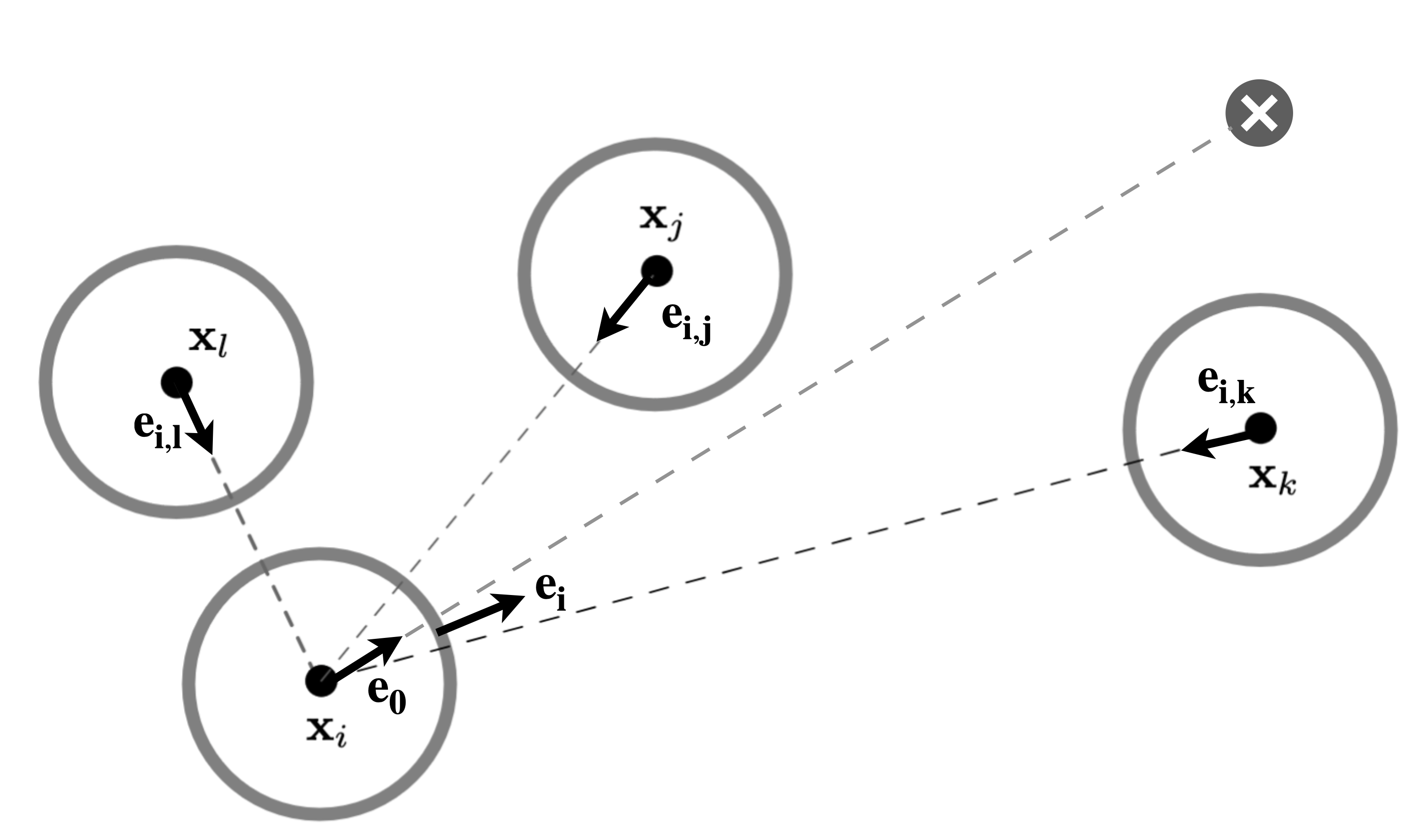
Calculation of the movement direction
This mathematical representation ensures that the pedestrians are able to adjust their speed and direction based on their interactions with neighboring agents, ultimately resulting in a collision-free movement.
$$\mathbf e_i(\mathbf x_i,\mathbf x_j,\ldots)=\frac{1}{N}\left(\mathbf e_0+\sum_j R(s_{i,j})\right)$$
with $\mathbf e_0$ the desired direction, $N$ a normalization constant such that $|\mathbf e_i|=1$ and $R(s)=a,\exp\big((l-s)/D\big)$ the repulsion function calibrated by the coefficient $a>0$ and distance $D>0$.
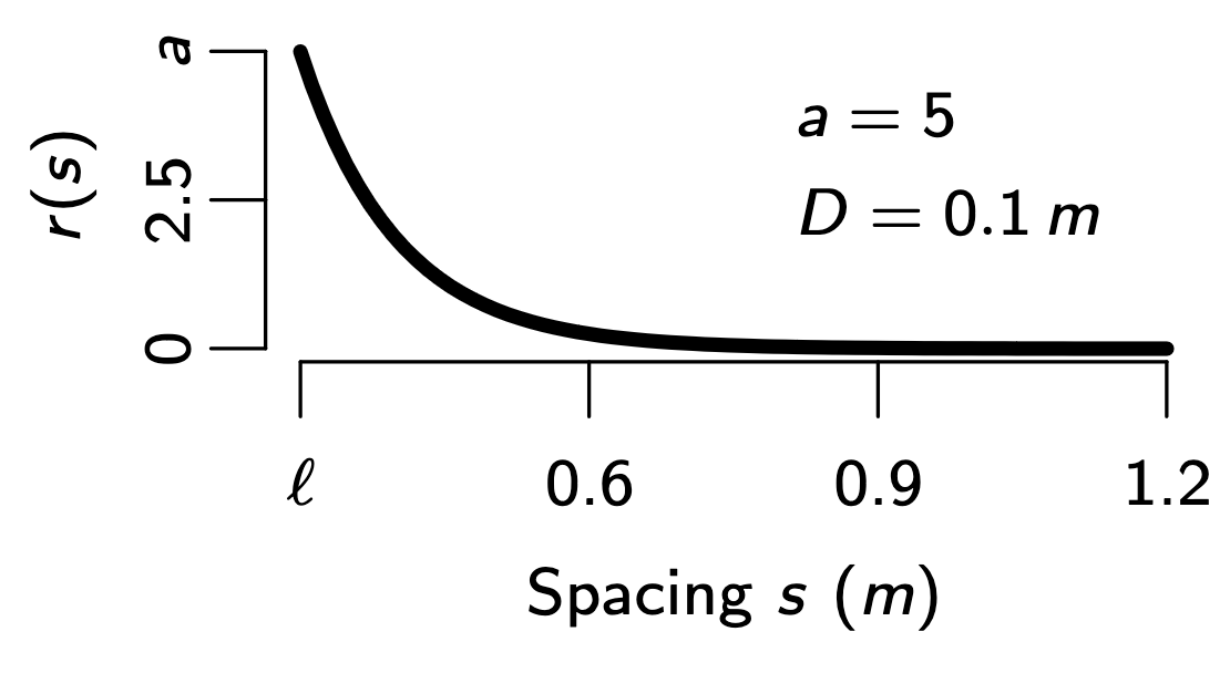
Repulsive influence in the direction
Speed function
The velocity is calculated by multiplying two functions: A speed function $V_i$ and a direction function $\textbf{e}_i$.
Inspired from car-following models, the speed function only depends on the distance to the nearest pedestrian or obstacle in front through an Optimal Velocity (OV) function.
The set $J_i$ of pedestrians and obstacles in front is given by
$$J_i=\big\{j,\mathbf e_i\cdot \mathbf e_{ij}\le 0\text{and}~|\mathbf e_i^\perp\cdot\mathbf e_{ij}|\le l/s_{ij}\big\}.$$
The distance to the nearest pedestrian or obstacle in front is then the minimum $$s_i=\min_{j\in J_i}s_{ij}.$$
In the following, the OV function is the piecewise linear $$V(s)=\min\big\{v_0,\max{0,(s-l)/T}\big\},$$
satisfies
$$\begin{align*}V(s)&\gt0\quad\forall s\gt l\\ V(s)&=0\quad\forall s\le\ell\end{align*}$$
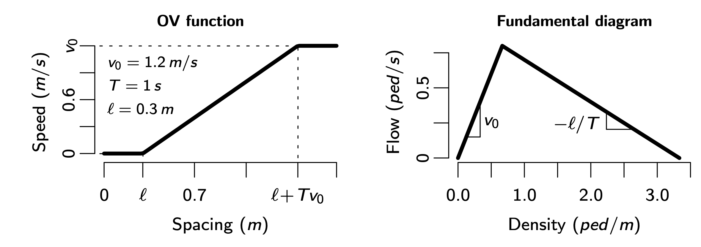
OV speed function vs fundamental diagram
The spacing is calculated along the direction of motion and is defined as the spacing to the nearest neighbor that may collide with the agent. See following picture:
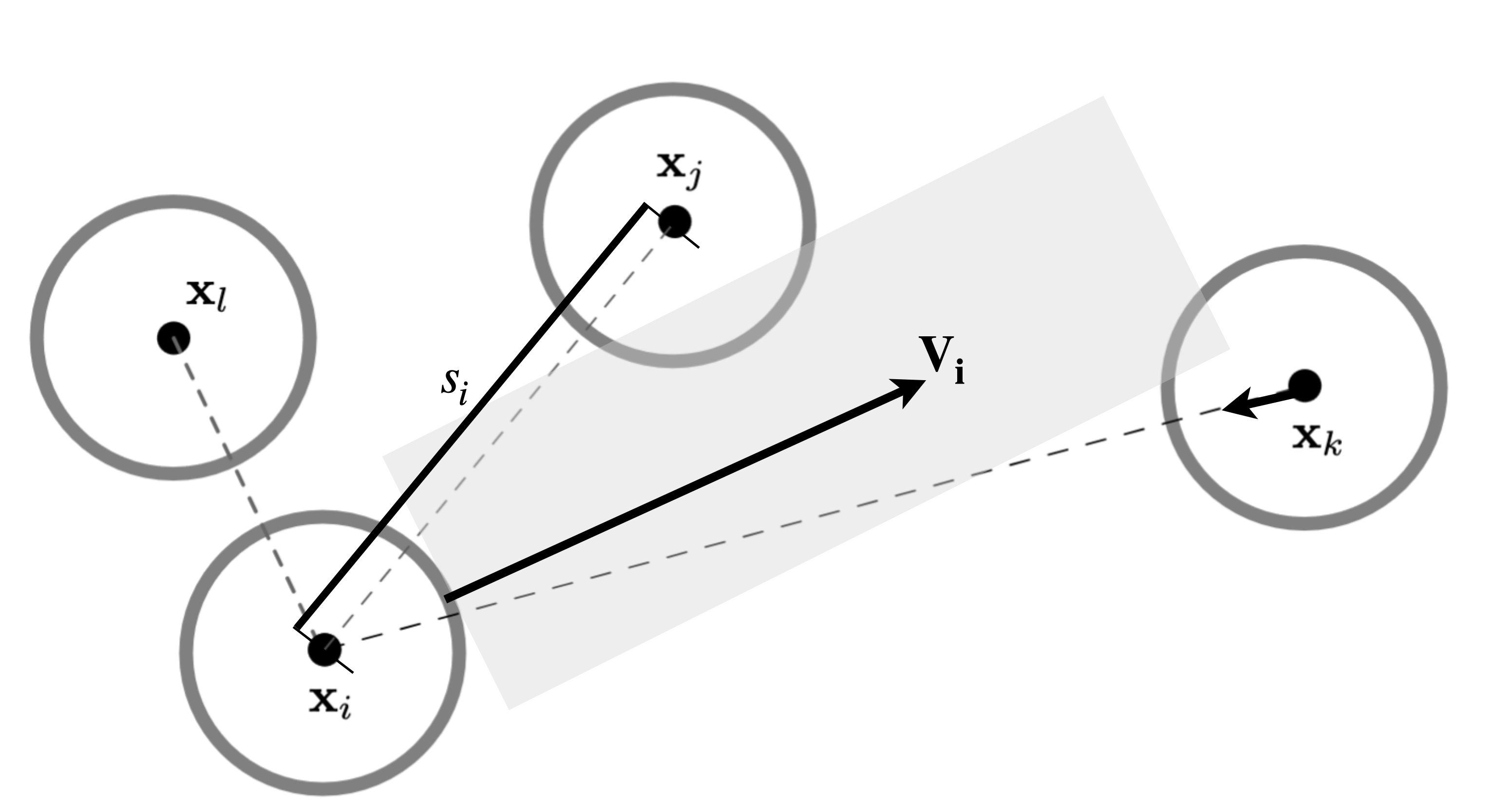
Calculation of the minimal speed in the direction of motion
Parameters
The collision-free speed model depends on five parameters:
- Pedestrian diameter ($l \ge 0$)
- Desired speed ($v_0 > 0$)
- Time gap ($T > 0$)
- Repulsion rate and distance ($a>0$ and $D>0$)
Limitations of the collision-free speed model
Despite its ability to simulate pedestrian dynamics and replicate real-world phenomena, the collision-free speed model has some limitations that should be acknowledged.
- Initially, the model operates on basic assumptions and might not encompass the intricate nuances of real pedestrian actions, particularly with its representation of agents as circles.
- It overlooks elements like response time and visual interpretation.
- The model may not represent stop-and-go dynamics in crowded regions or gridlocks aptly, unless manifested in confined bottlenecks with a circular form.
- The model does not take into account other influencing variables like obstacles or environmental conditions that could impact pedestrian movement.
Numerous studies have presented different enhancements to the collision-free speed-based pedestrian model with the aim of addressing its limitations and improving the accuracy of pedestrian simulations. For instance, Xu [2] proposed a comprehensive velocity model that takes into account wall influence and incorporates velocity-based ellipses for accurate distance calculations. Moreover, improvements were made to the direction function in order to ensure seamless changes in pedestrian directions during simulation. Similarly, other researchers such as [3], [4], and [5] introduced additional refinements to enhance the direction function further.
Challenges in Implementing Collision Free Speed Models
Numerical solution of the first-order ordinary differential equation defined by the model is solved as follows:
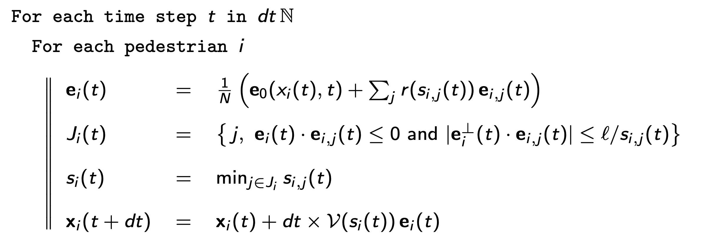
Update algorithm
The implementation of collision-free speed models presents several challenges. One challenge is the lack of definition for agent-wall interactions in the original model. However, this issue has been tackled by proposed enhancements to the model, such as Xu’s generalized velocity model. Another challenge lies in accurately calibrating the parameters in both the speed and direction models. In certain symmetrical scenarios, determining a well-defined direction function can be difficult.
Isotropical direction influence
The direction model is uniform, meaning it does not differentiate between various directions of influence. The model treats all directions equally and does not consider specific pedestrian preferences or biases in their movement. This may lead to certain unrealistic situations where the agent’s direction is influenced by agents from behind them.
Balancing Collision Avoidance with Performance: Selecting the Appropriate Time-Step
The continuous definition of the model is proved to be collision-free in any situation. However, the discretisation of the model, as often required for computational efficiency, can introduce potential collision problems. While the speed model has a fast and efficient implementation, it is crucial to select a sufficiently small time step when solving the ordinary differential equation with Euler scheme in order to ensure that the model remains collision-free. Therefore, the model is collision-free in discrete time if
$$\delta t \le \min\left\{\frac T2,\frac{l(\sqrt2-1)}{v_0\sqrt2}\right\}$$
The condition for collision-free dynamics is determined solely by the parameters of the speed model. For example, if we use parameter values of $T=1$ s, $v_0=1.2$ m/s and $l$, with a smallness condition on the time step approximate to $\delta t \le0.072$ s for explicit Euler schemes and circular pedestrian shape.
Parameter calibration
Additionally, accurately calibrating the repulsion rate and distance in the direction model can prove challenging due to variation based on specific environmental conditions and crowd dynamics.
References
[1] Tordeux, A., Chraibi, M., Seyfried, A. (2016). Collision-Free Speed Model for Pedestrian Dynamics. In: Knoop, V., Daamen, W. (eds) Traffic and Granular Flow ‘15.
https://doi.org/10.1007/978-3-319-33482-0_29[2] Xu, Q., Chraibi, M., Tordeux, M., Zhang (2019). Generalized collision-free velocity model for pedestrian dynamics. Physica A: Statistical Mechanics and its Applications, Volume 535.
https://doi.org/10.1016/j.physa.2019.122521[3] Rzezonka, J., Chraibi, M., Seyfried, A., Hein, B., Schadschneider, A. (2022). An attempt to distinguish physical and socio-psychological influences on pedestrian bottleneck. Royal Society Open Science.
https://royalsocietypublishing.org/doi/10.1098/rsos.211822[4] Zhang, S., Zhang, J., Chraibi, M., Song, W. (2021). A speed-based model for crowd simulation considering walking preferences. Communications in Nonlinear Science and Numerical Simulation, Volume 95.
https://doi.org/10.1016/j.cnsns.2020.105624[5] Xu, Q., Chraibi, M., Seyfried, A. (2021). Anticipation in a velocity-based model for pedestrian dynamics. Transportation Research Part C: Emerging Technologies, Volume 133.
https://doi.org/10.1016/j.trc.2021.103464[6] Tordeux, A. talk in TGF15, Delft.
Slides.